NEWVectors or files. Pick a path.Start →

    Diagrams

    How multimodal search actually works, one picture at a time. Each diagram explains a single idea: from what an embedding is, to why reranking exists, to how the whole extract → index → retrieve loop fits together.
    All (64)
    IR Foundations(18)
    Diagram Series(46)
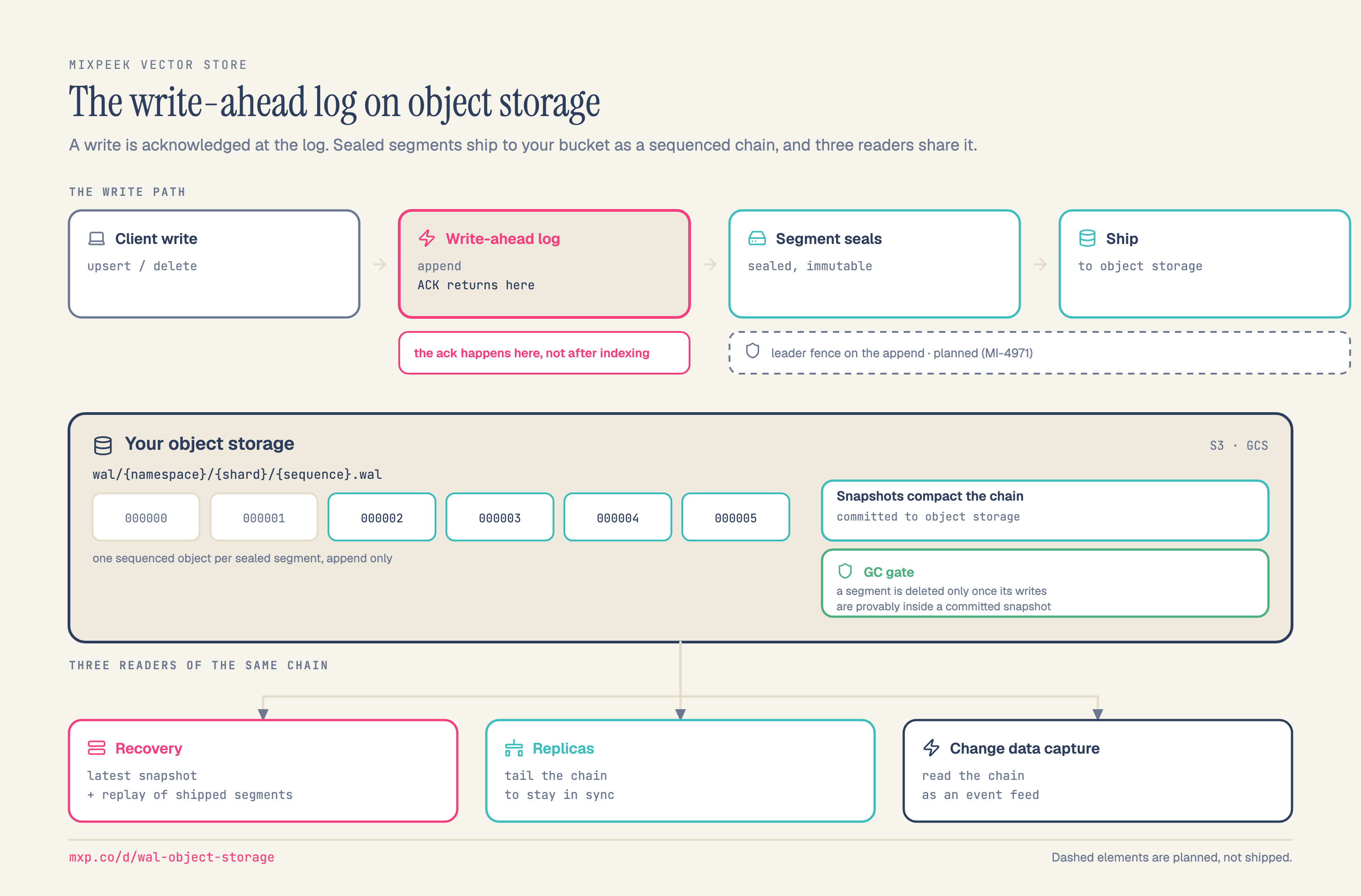
    A three-band architecture diagram of the Mixpeek Vector Store write path on object storage. The top band runs left to right: a client write of an upsert or delete, into a write-ahead log where the append happens and the acknowledgement returns, then a segment sealing as immutable, then shipping to object storage. A callout under the log reads that the acknowledgement happens there and not after indexing, and a dashed box spanning the seal and ship steps marks a leader fence on the append as planned rather than shipped. The middle band is your object storage, an S3 or GCS bucket holding one sequenced object per sealed segment at the path wal slash namespace slash shard slash sequence dot wal, drawn as a row of numbered segments with the two oldest greyed. Beside them, snapshots compact the chain and commit to object storage, and a garbage-collection gate states that a segment is deleted only once its writes are provably inside a committed snapshot. The bottom band fans out to three readers of the same chain: recovery, which takes the latest snapshot plus a replay of shipped segments; replicas, which tail the chain to stay in sync; and change data capture, which reads the chain as an event feed.
    Architecture

    Write-Ahead Logs on Object Storage: The MVS Write Path

    The acknowledgement happens at the log, before indexing. Everything downstream reads the same sequenced chain of objects in your own bucket.
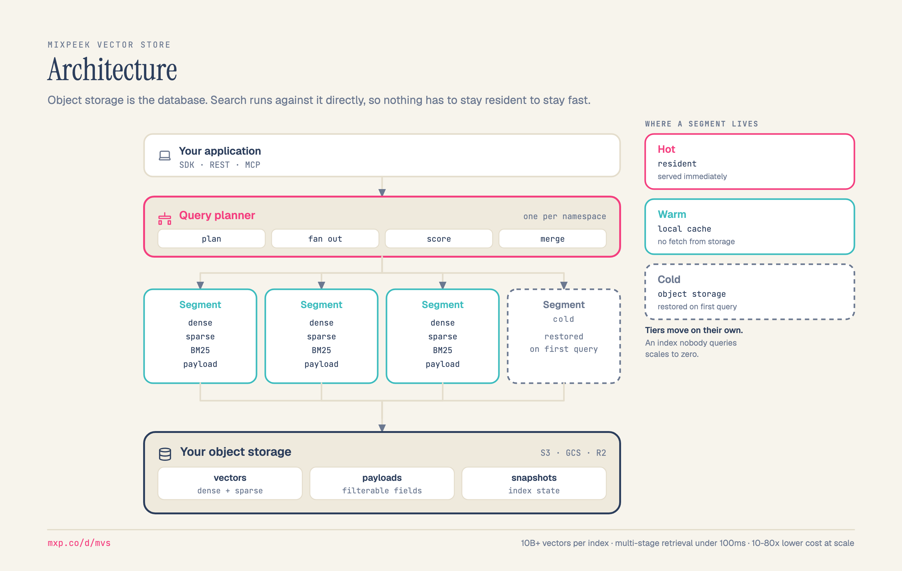
    A layered architecture diagram of the Mixpeek Vector Store. Tiers move on their own and an index nobody queries scales to zero: a right-hand rail shows where a segment lives, hot and resident, warm in local cache, or cold in object storage. The main flow runs top to bottom. Your application reaches MVS over SDK, REST or MCP and feeds a query planner that runs one per namespace and does plan, fan out, score and merge. The planner fans out to four segments; three are active and each carries dense, sparse, BM25 and payload, while the fourth is drawn dashed as a cold segment restored on first query. All four converge on your object storage, an S3, GCS or R2 bucket holding vectors, payloads and index snapshots.
    Product

    MVS Architecture: Object Storage Is the Database

    Object storage is the database. A query planner fans out across segments and merges, and the segments themselves are cheap to drop because the bucket already holds everything they need.
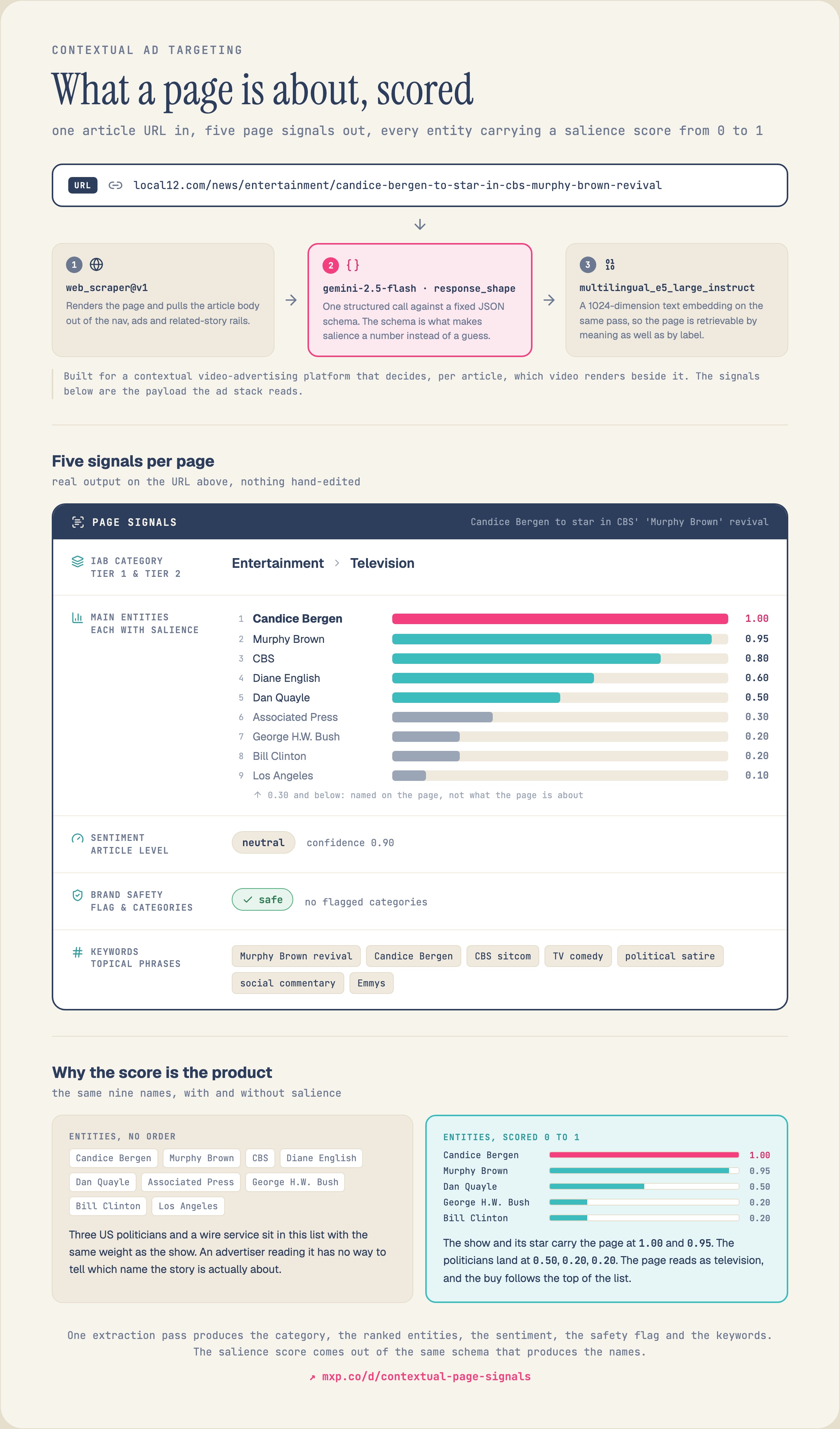
    One article URL producing five structured signals: IAB category at tier 1 and tier 2, main entities each carrying a salience score from 0 to 1 drawn as a ranked bar chart, article-level sentiment, a brand-safety flag with categories, and keywords. A side panel contrasts a flat entity list against the same entities scored.
    Retrieval Mechanics

    Contextual Page Signals: Scoring Entities Instead of Listing Them

    Nine entities come off one local-news page, three of them US politicians. Flat, it reads as a politics page. Scored, the top two are the actress and the sitcom and it is obviously a television story.
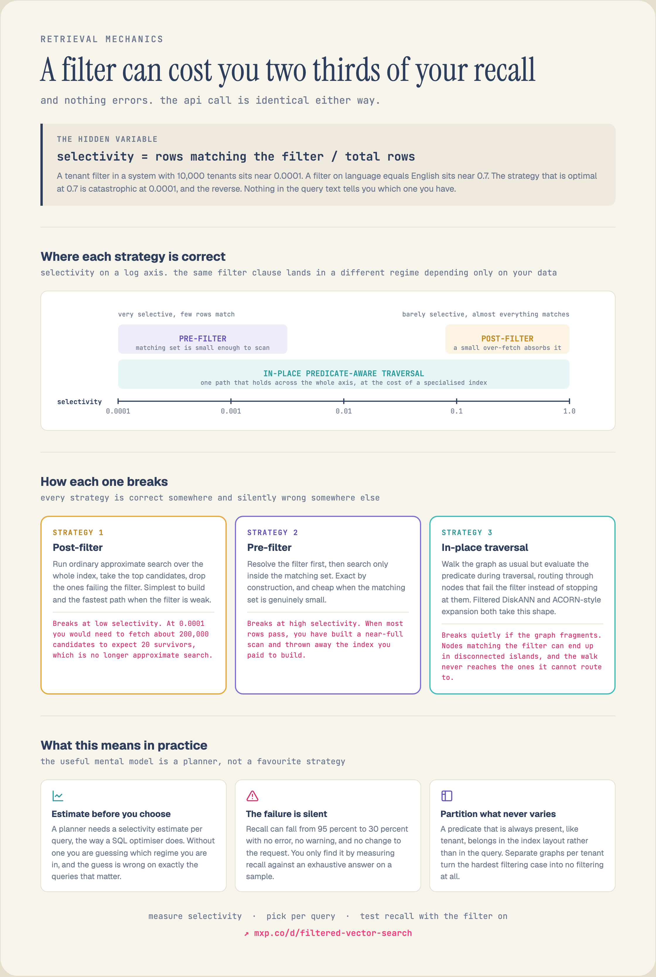
    Diagram of filtered vector search showing how filter selectivity decides which of three strategies works: pre-filtering, post-filtering, and single-stage filtered traversal, with the failure each one hits at the wrong selectivity.
    Retrieval Mechanics

    Filtered Vector Search: Why the Same Filter Is Free or Fatal

    Adding a filter to a vector search looks like a WHERE clause. Selectivity decides whether it costs nothing or destroys your results, and the API call is identical either way.
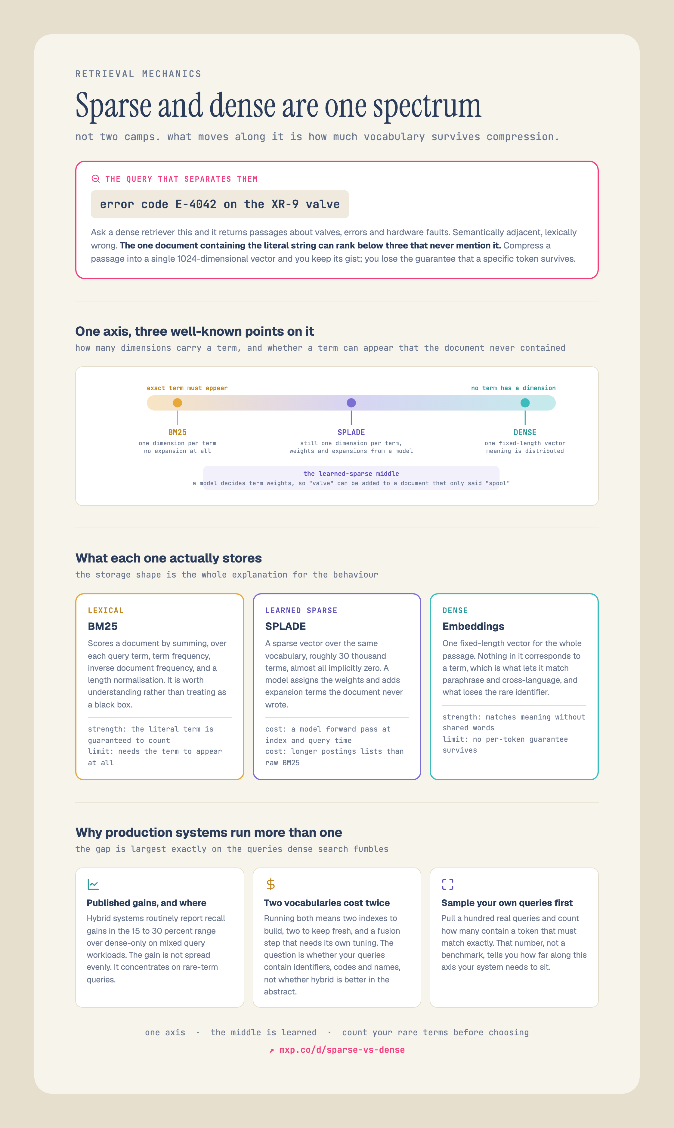
    Diagram placing BM25, SPLADE and dense embeddings on a single axis measuring how much vocabulary survives compression, with what each one stores and why production systems run more than one.
    Retrieval Mechanics

    Sparse and Dense Are One Spectrum, Not Two Camps

    BM25, SPLADE and dense embeddings sit on one axis. What moves along it is how much vocabulary survives compression, which is why a rare identifier ranks below three passages that never mention it.
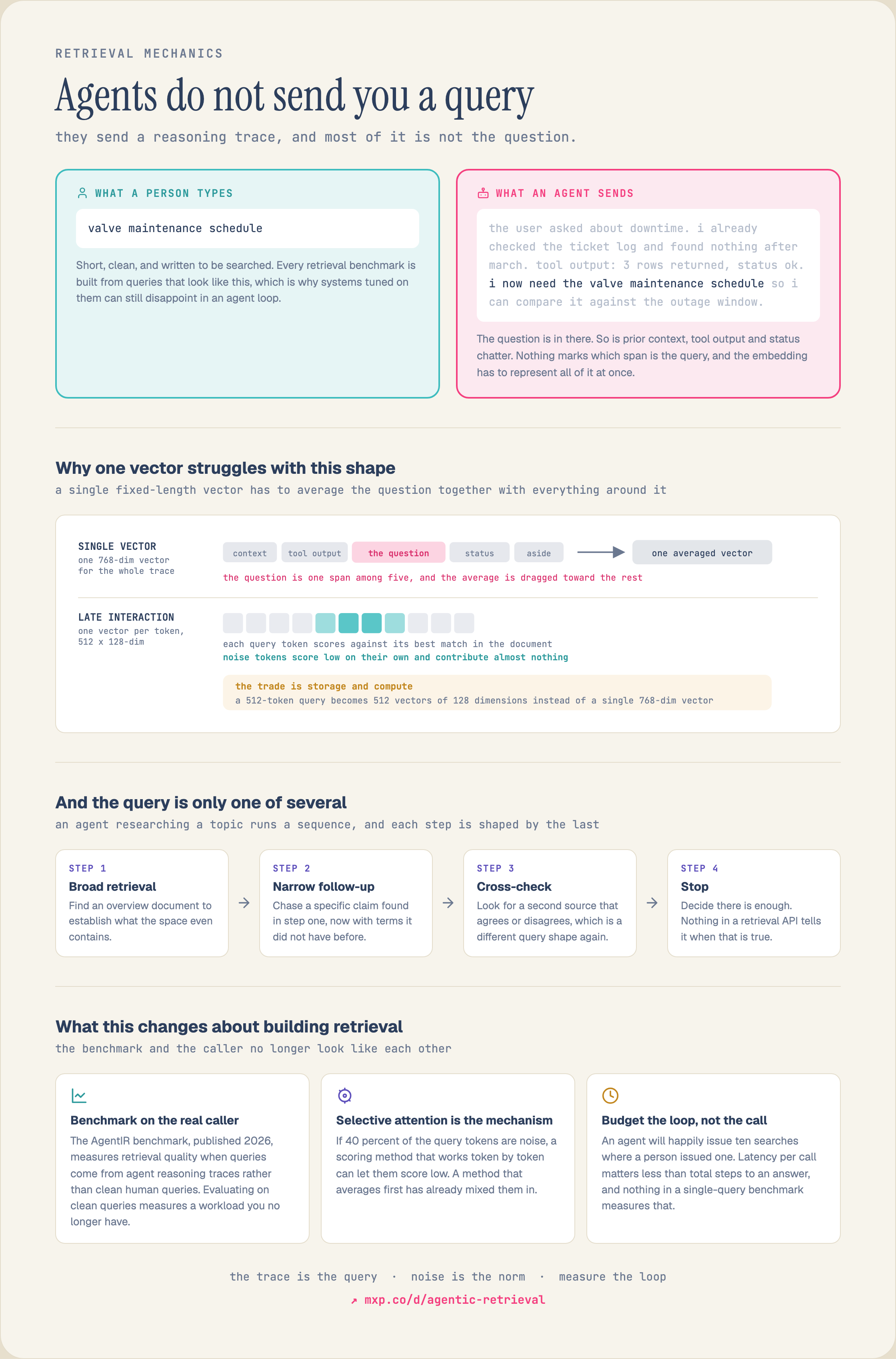
    Diagram contrasting a human query with an agent query, showing how agent calls carry accumulated state and prior tool output, and what a retrieval layer must return differently as a result.
    Retrieval Mechanics

    Agentic Retrieval: What Changes When the Caller Is Not a Person

    A person types four words. An agent sends its accumulated state, prior tool output and the reason it is asking. The retrieval layer is answering a different kind of caller.
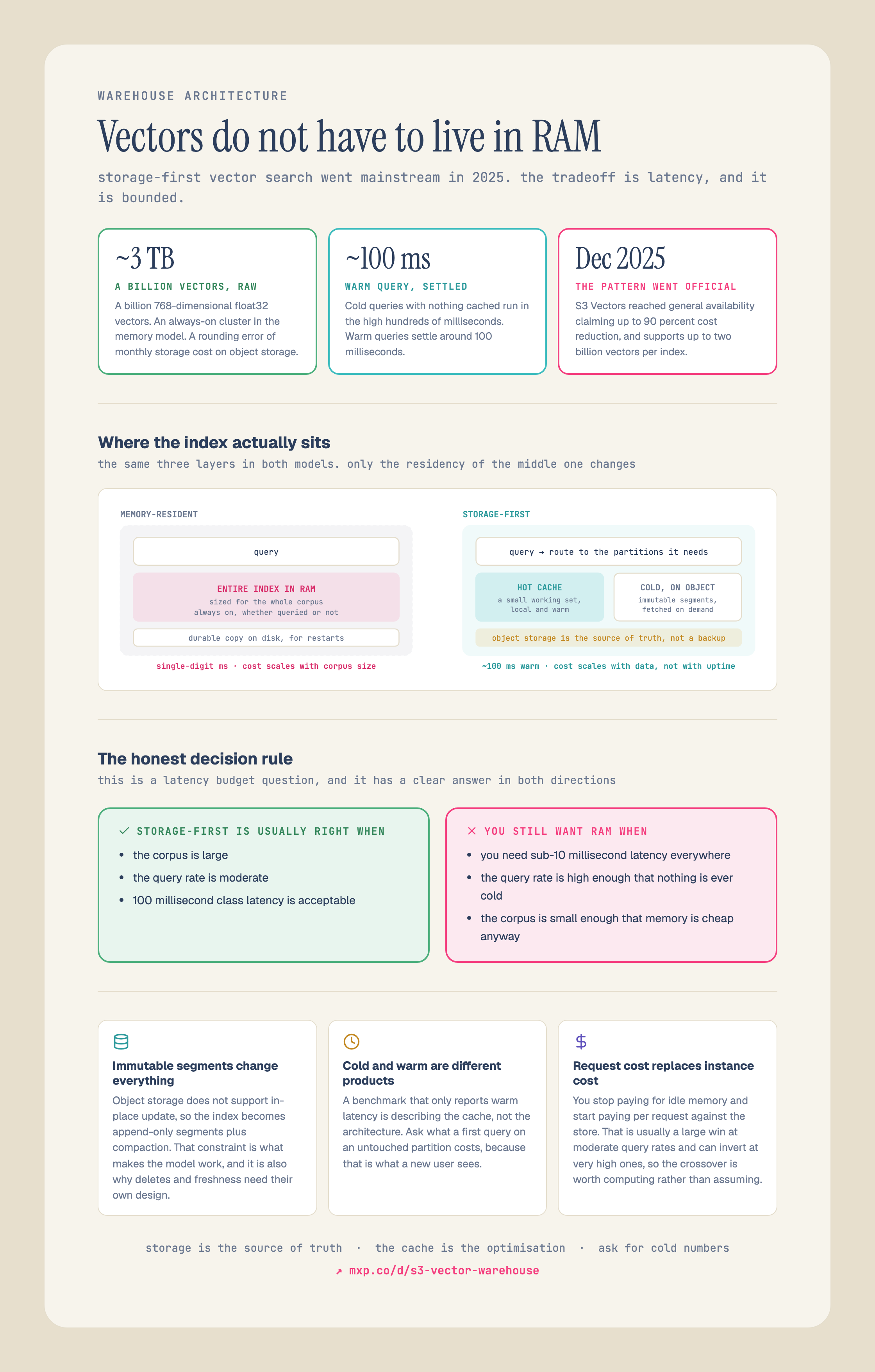
    Diagram comparing memory-resident vector search against storage-first vector search on object storage, showing the cost structure of a billion 768-dimensional vectors under each model.
    Architecture

    The S3 Vector Warehouse: Storage-First Vector Search

    A billion 768-dimensional float32 vectors is about 3TB raw. Memory-resident, that is a cluster running whether anyone queries it or not. On object storage it is a rounding error of monthly storage.
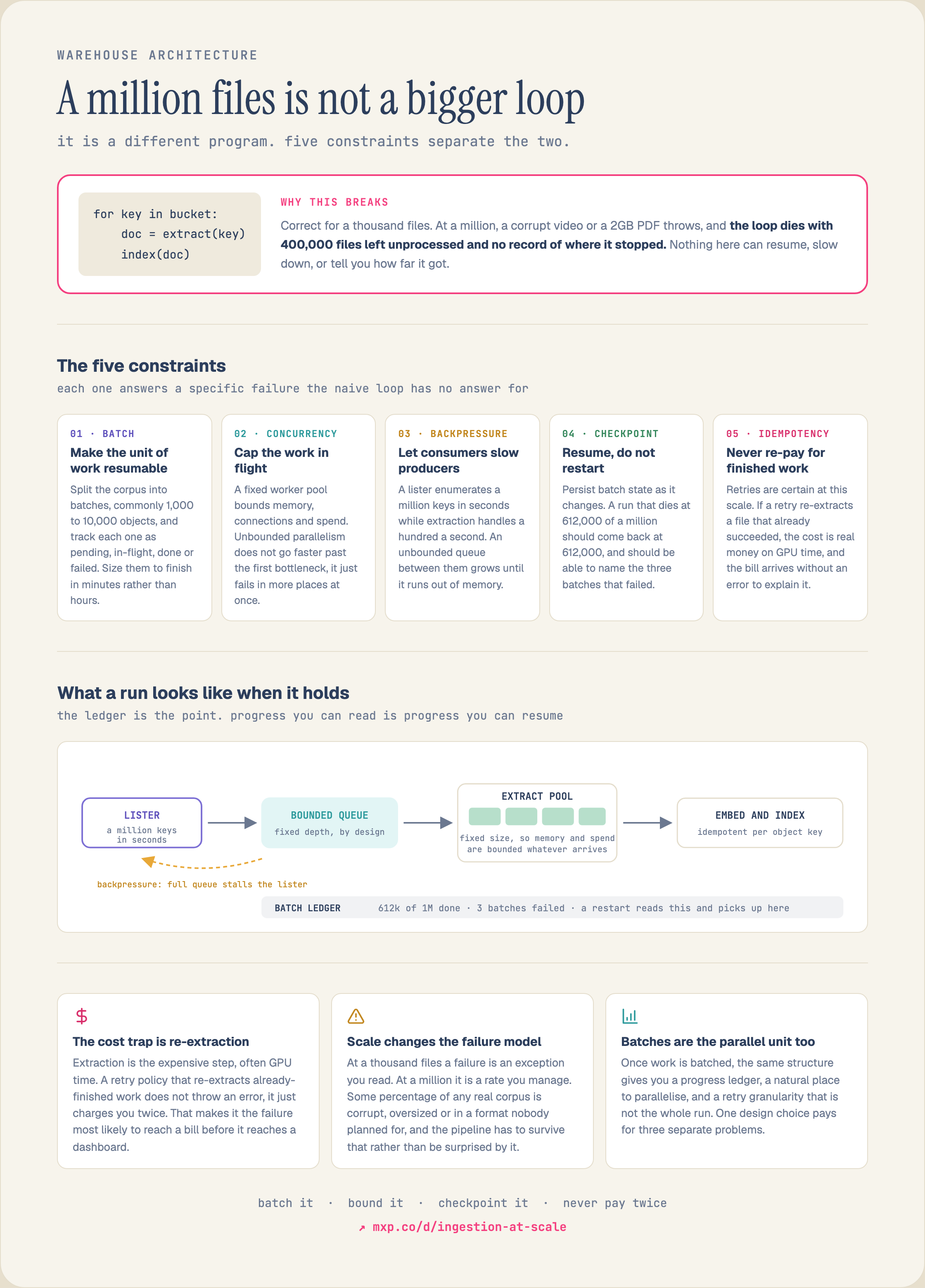
    Diagram showing why a naive for-each ingestion loop fails at scale, and the checkpointing, isolation and retry structure that replaces it.
    Architecture

    Ingestion at Scale: Why the Obvious Loop Dies at a Million Files

    The obvious loop is correct for a thousand files. At a million, one corrupt video kills it with 400,000 files unprocessed and no record of where it stopped.
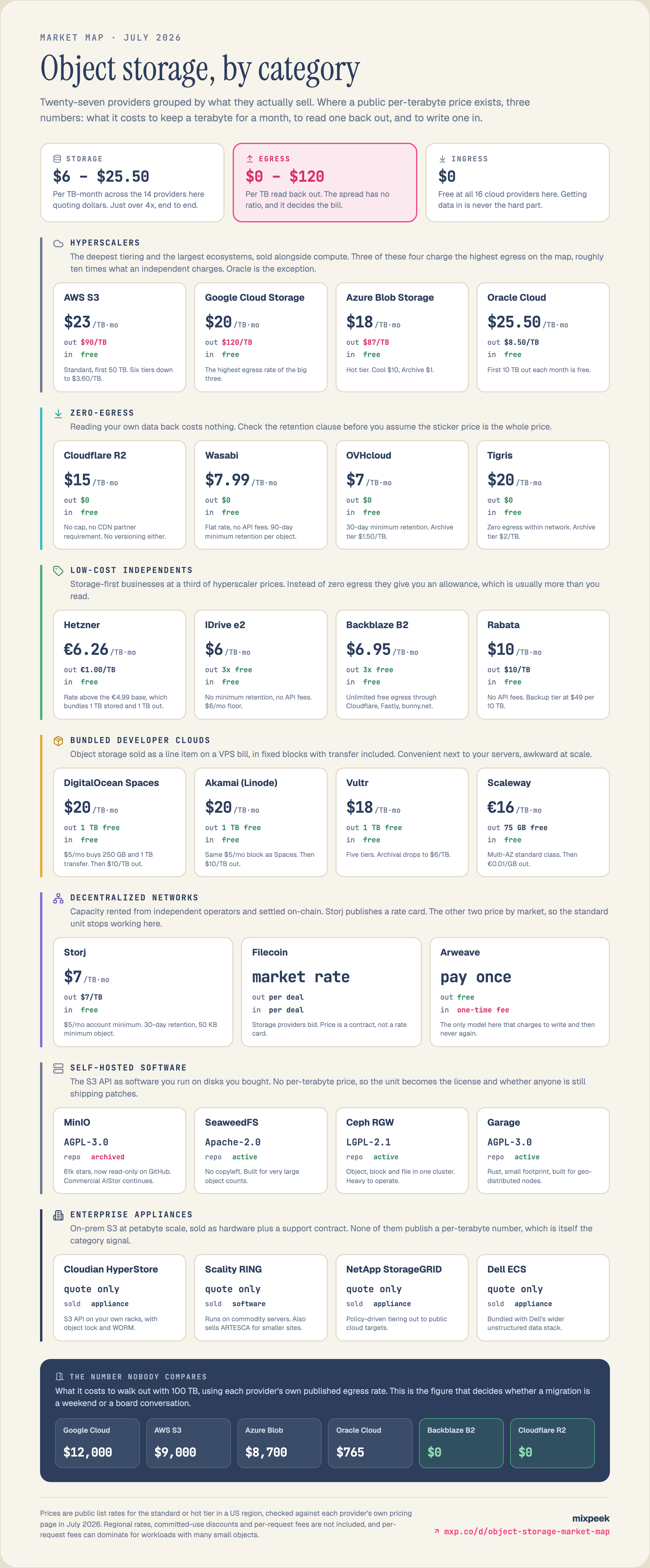
    Market map of 27 object storage providers across seven categories (hyperscalers, zero-egress, low-cost independents, bundled developer clouds, decentralized networks, self-hosted software, enterprise appliances), each showing storage cost per TB-month, egress cost per TB, and ingress cost, with a closing panel pricing the cost of moving 100 TB out of each major provider.
    Market Maps

    The Object Storage Market Map: 27 Providers, Priced

    27 object storage providers across seven categories, each carrying storage $/TB-month, egress $/TB, and ingress. The closing panel prices what it costs to walk out with 100 TB.
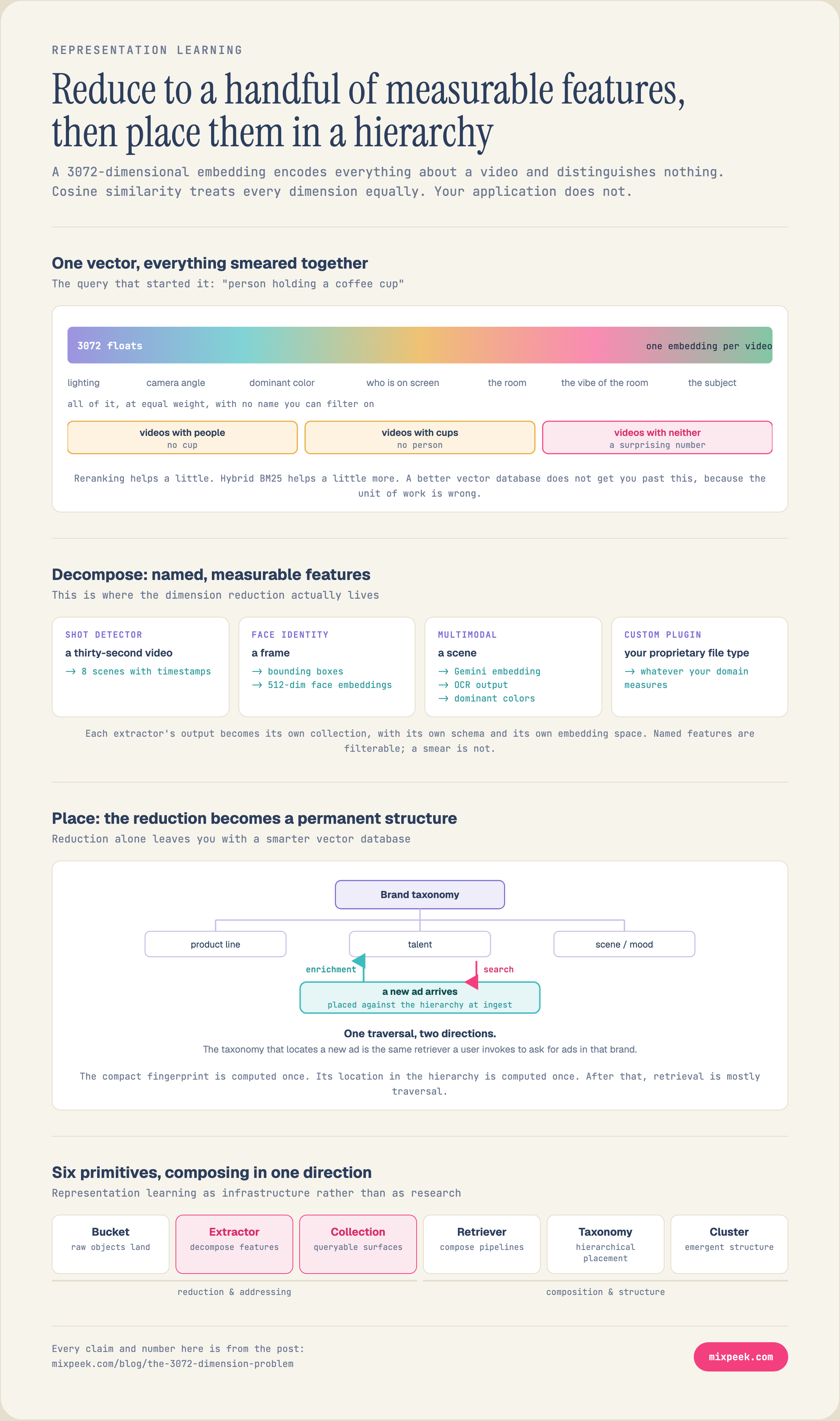
    A 3072-dimensional embedding encodes everything about a video and distinguishes nothing: lighting, camera angle, dominant color, who is on screen, the room and the vibe of the room are all smeared across the same floats at equal weight, with no name you can filter on. That is why a search for a person holding a coffee cup returns videos with people, videos with cups, and a surprising number with neither, and why reranking and hybrid BM25 each help only a little. Decomposition is where the dimension reduction actually lives: a shot detector turns a thirty-second video into eight scenes with timestamps, a face identity model turns a frame into bounding boxes and 512-dimension face embeddings, a multimodal extractor turns a scene into a Gemini embedding plus OCR output plus dominant colors, and a custom plugin does the same for a proprietary file type. Each extractor's output becomes its own collection with its own schema and its own embedding space, so the features are named and filterable where a smear is not. Reduction alone leaves a smarter vector database; the leverage is placement. A new ad is placed against a brand taxonomy at ingest, and because the taxonomy that locates it is the same retriever a user invokes to ask for ads in that brand, enrichment and search become one traversal in two directions. Six primitives compose in one direction: bucket, extractor, collection, retriever, taxonomy, cluster.
    IR Foundations

    The 3072-Dimension Problem: Reduce, Then Place

    Representation learning as infrastructure: reduce to named features, then make the reduction a permanent, queryable hierarchy.

    An ordinary embedding model spreads information across all dimensions with no ordering guarantee, so dimension 900 may carry as much signal as dimension 5 and truncating the vector discards random pieces of meaning. Matryoshka Representation Learning changes the objective so the model packs the most general information into the front of the vector and progressively finer detail toward the back, which makes every prefix a complete usable coordinate. The nesting is drawn as five bars that all start at dimension 0 and grow: the first 64 dimensions carry coarse semantics, enough to tell a cat photo from a car photo; 128 is the prefix the retrieval cascade indexes the whole corpus at; 256 gives mid resolution, enough to separate breeds of cat or a refund request from a refund confirmation; and the full 1024 gives fine resolution for ranking near-duplicates. The mechanism is a modified loss rather than a special architecture: one forward pass produces one d-dimensional output, the training loss is computed independently at each prefix size in the set 64, 128, 256, 512, 1024, and those losses are summed, so the front of the vector has to work on its own. What it buys is a retrieve-coarse, rerank-fine cascade: index 10,000,000 items at a 128-dimension truncation costing 5.1 GB instead of the full 41 GB, retrieve a top-200 shortlist with the truncated query, fetch the full 1024-dimension vectors for those 200 candidates only, and return a final top 10.
    IR Foundations

    Matryoshka Representation Learning: One Vector, Five Resolutions

    Why an agent can search a corpus coarsely and still rank the winners precisely, without re-embedding anything.
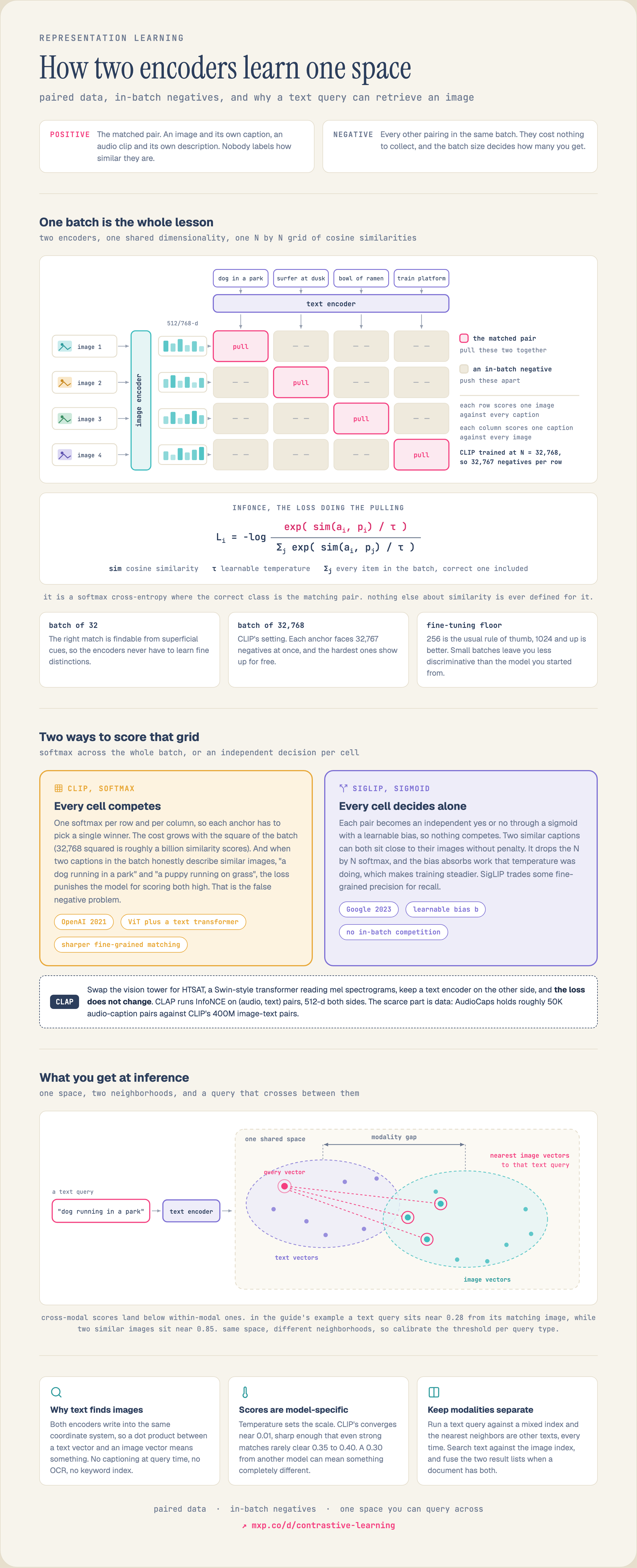
    Contrastive learning trains a model to answer one question: are these two things related? You give it a batch of N anchor-positive pairs (an image and its own caption for CLIP, an audio clip and its description for CLAP) and nobody ever labels how similar a pair is, because the pairing itself is the entire supervision signal. Inside one batch each anchor has one positive and N-1 negatives, since every other item is by definition a non-match. CLIP scores the batch as an N by N grid of cosine similarities where the diagonal holds the true pairings, and InfoNCE pulls the diagonal together while pushing everything off it apart. Batch size is therefore a first-class hyperparameter rather than a throughput knob: CLIP trained at 32,768 so each anchor faced 32,767 simultaneous negatives and could not win on coarse cues. CLIP uses a softmax over the batch, SigLIP replaces it with a pairwise sigmoid that needs no global normalization and so trains stably at large scale.
    IR Foundations

    Contrastive Learning: How Two Encoders Learn One Space

    Why a text query can retrieve an image: the pairing is the only supervision.
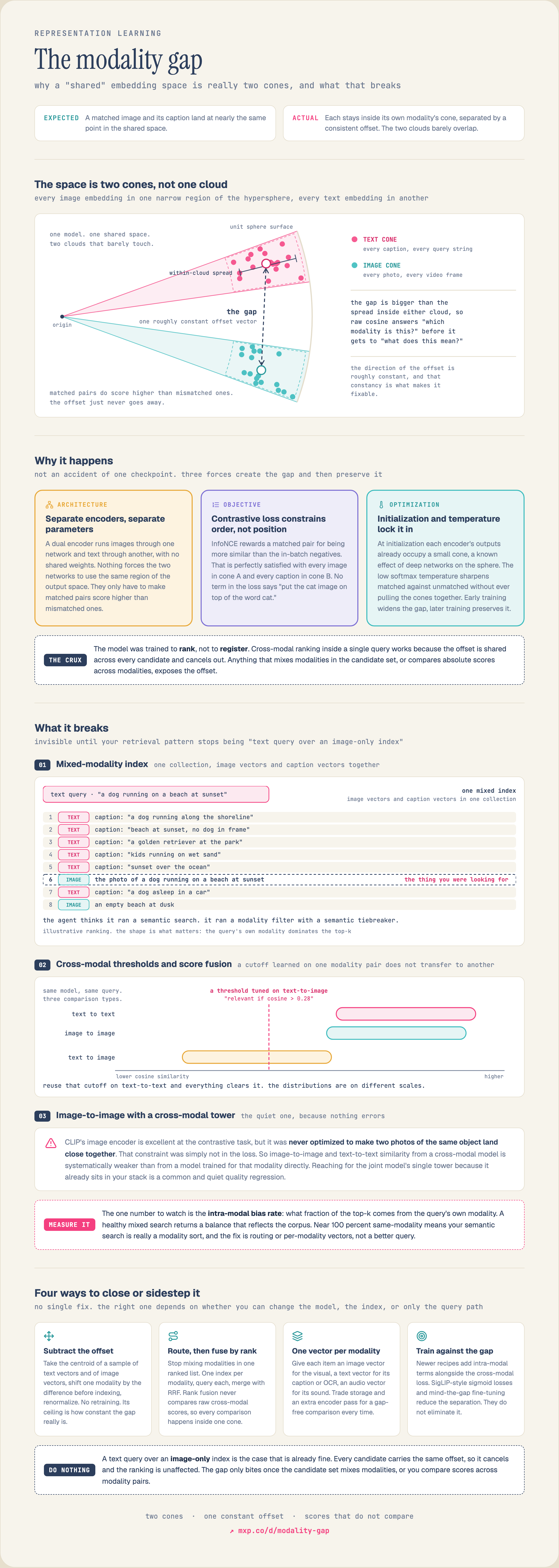
    Train a dual encoder like CLIP and you would expect a matched image and its caption to land at nearly the same point in the shared space. They do not. All image embeddings occupy one narrow cone of the hypersphere and all text embeddings occupy a different, well-separated cone, and the two clouds barely overlap. A matched pair is closer to each other than to mismatched pairs, but both still sit inside their own modality's region, separated by a roughly constant offset vector. Three forces create and preserve it: a dual encoder runs each modality through a separate network with no shared weights, InfoNCE only requires a matched pair to outscore in-batch negatives which is satisfied with every image in cone A and every caption in cone B, and at initialization each encoder's outputs already occupy a small cone while a low softmax temperature sharpens matched against unmatched pairs without pulling the cones together. The model was trained to rank, not to register.
    IR Foundations

    The Modality Gap: A Shared Space Is Really Two Cones

    Why cross-modal retrieval underperforms same-modality retrieval in one shared space.

    Every relevance score in retrieval comes from one of three architectures, and they differ on exactly one axis: when the query is allowed to see the document. A bi-encoder never lets them meet until the end, encoding query and document separately into one vector each and scoring by cosine, so document vectors are computed once at index time and search is an ANN lookup, but the encoder had to guess what mattered before the question existed. A cross-encoder lets them meet immediately, concatenating query and document so every query token attends to every document token, which is worth 5 to 15% on benchmarks but costs quadratic time per pair and can only rerank a shortlist. Late interaction keeps a vector per token, computes the interaction at query time with MaxSim (each query token takes its best match in the document, then sum), and pays for it in storage: hundreds of vectors per document instead of one.
    MUVERA / Multi-Vector

    Three Ways to Score a Query Against a Document

    Bi-encoder, cross-encoder, late interaction: when the query is allowed to see the document.
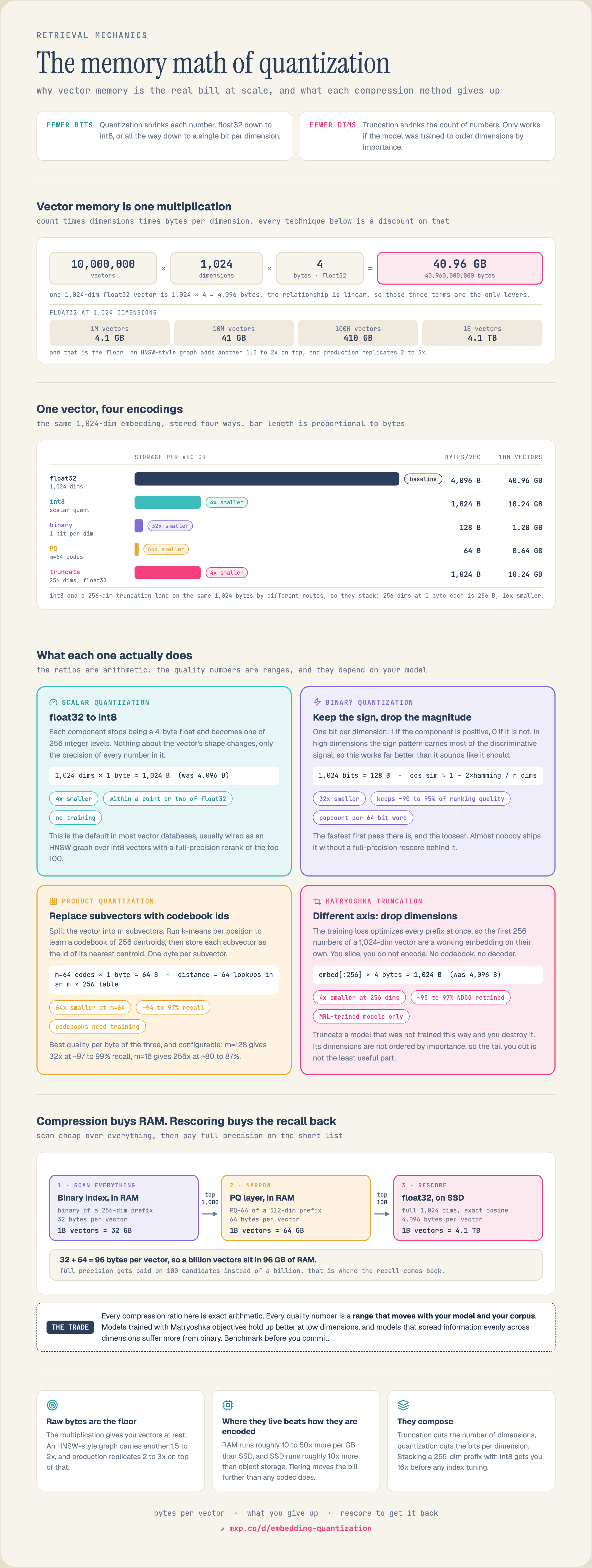
    Vector memory is one multiplication: bytes equals vectors times dimensions times bytes per dimension. At 1,024 dimensions in float32 that is 4,096 bytes per vector, so 10 million vectors is 40.96 GB and a billion is 4.1 TB. The relationship is linear, which means there are exactly three levers and every compression technique is a discount on one of them. int8 quantization scales each dimension into a byte for a 4x cut, binary quantization keeps only the sign of each dimension for 32x, product quantization splits the vector into subvectors and replaces each with a centroid id for arbitrary ratios, and Matryoshka truncates dimensions because the model was trained so the first d dimensions are themselves a valid embedding. The rescore cascade is what makes any of it survivable: retrieve wide with the cheap representation, then re-rank the shortlist with a more precise one.
    IR Foundations

    The Memory Math of Quantization

    Every compression method is a discount on one term of vectors x dimensions x bytes.
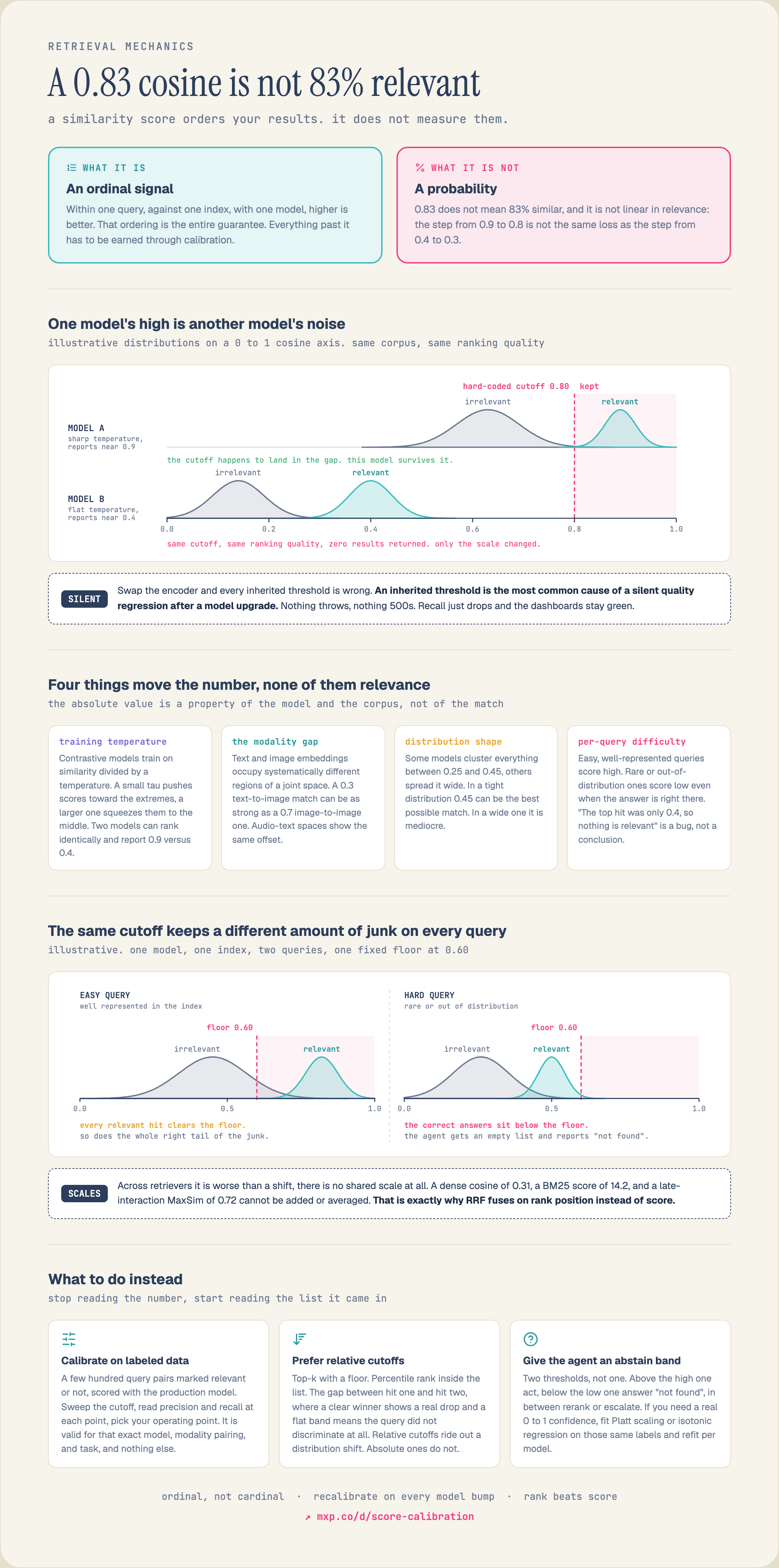
    A similarity score is an ordinal signal. Within one query, against one index, with one model, higher is better, and that ordering is the entire guarantee. A cosine of 0.80 does not mean 80% similar, and the score is not linear in relevance either: the step from 0.9 to 0.8 is not the same loss as the step from 0.4 to 0.3. Four independent effects shape the absolute value and none is about whether the result is relevant. Training temperature: contrastive models divide similarity by a temperature, so two models can rank identically while one reports around 0.9 and the other around 0.4. The modality gap: a 0.3 text-to-image match can be as strong as a 0.7 image-to-image one. Distribution shape: some models cluster everything between 0.25 and 0.45, where 0.45 is the best possible match. And per-query difficulty: a rare query scores lower even when the right answer is first.
    IR Foundations

    A 0.83 Cosine Is Not 83% Relevant

    Scores are ordinal, not cardinal, which is why a fixed threshold silently breaks.

    The unstructured-data problem: the large majority of enterprise data is unstructured (video, images, audio, and documents) that keyword systems and relational databases cannot search by meaning until it is turned into embeddings and indexed. The raw files are stored but not answerable.
    IR Foundations

    99% of your data has no rows

    Most enterprise data is unstructured: unsearchable by meaning until it is extracted, embedded, and indexed.
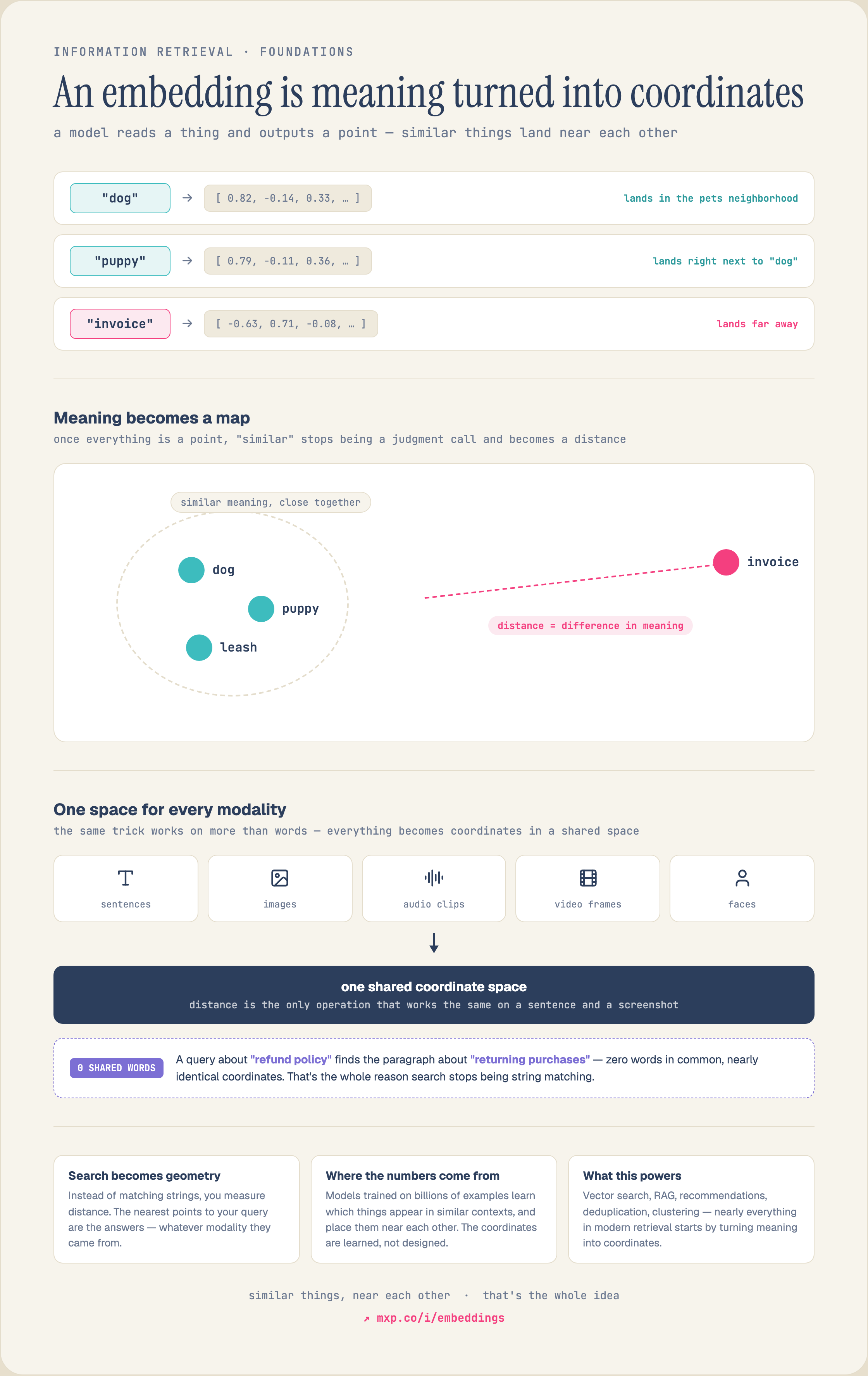
    An embedding turns meaning into coordinates: a model reads 'dog', 'puppy', and 'invoice' and outputs vectors, so 'dog' and 'puppy' land near each other while 'invoice' lands far away. Text, images, audio clips, video frames, and faces all map into one shared coordinate space where distance measures difference in meaning.
    IR Foundations

    An embedding is meaning turned into coordinates

    An embedding turns meaning into coordinates: similar things land near each other, across every modality.
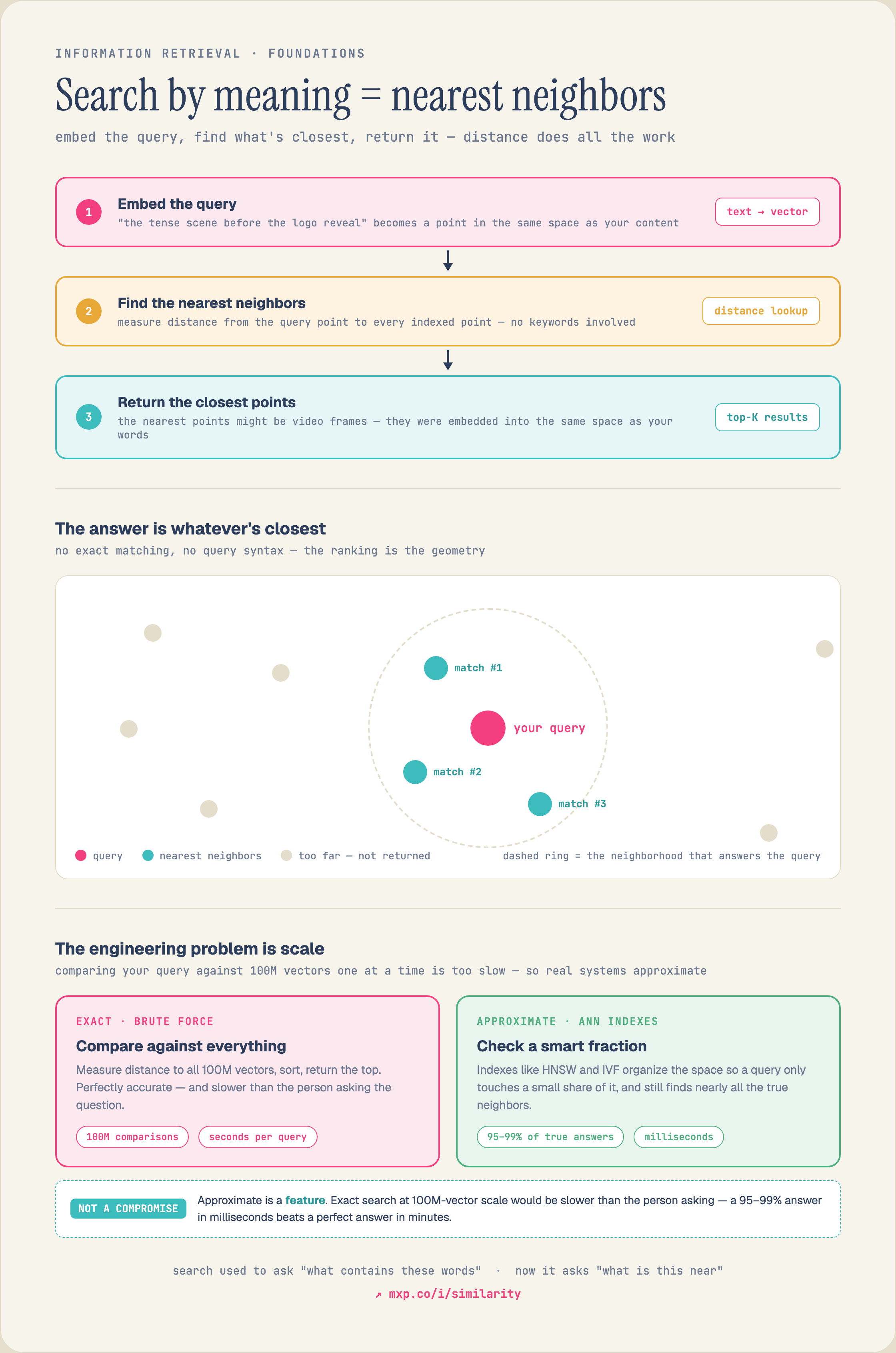
    Semantic search as nearest-neighbor lookup: embed the query into the same vector space as your content, measure distance to every indexed point, and return the closest top-K results with no keyword matching. Exact brute-force compares against everything and is accurate but slow, while approximate nearest-neighbor (ANN) indexes like HNSW and IVF check a smart fraction of the space and return 95-99% of true answers in milliseconds.
    IR Foundations

    Search by meaning = nearest neighbors

    Search by meaning is a nearest-neighbor lookup: embed the query, return the closest points.

    Object decomposition: you search inside the file, not for it. A one-hour recording.mp4 is split into scenes (visual embeddings), speech (transcript embeddings on silence and speaker turns), faces (who appeared and when), and on-screen text (OCR of slides and captions). A whole file being findable is not the same as usable: the thing you need is a moment inside it, like 23,41 where the renewal number is spoken while the pricing slide is on screen. The same move works on video, PDFs, and audio: one file becomes dozens of small, independently searchable documents.
    IR Foundations

    You search inside the file, not for it
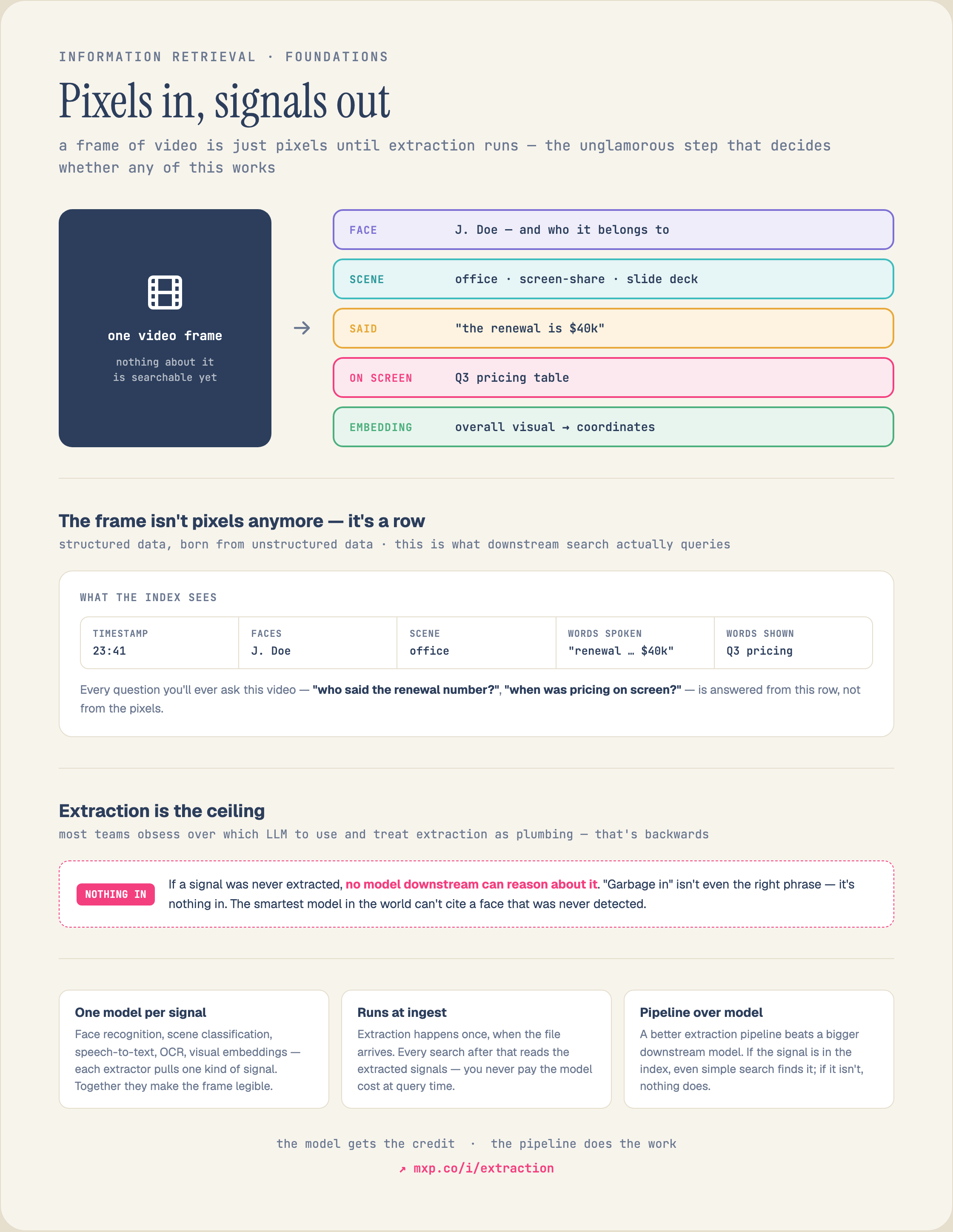
    You search inside the file, not for it

    Feature extraction turns raw pixels into searchable signals: one video frame becomes a structured row, face, scene, spoken words (transcript), on-screen text (OCR), and a visual embedding. Every question you later ask the video is answered from these extracted signals, not from the raw pixels; if a signal was never extracted, nothing downstream can search it.
    IR Foundations

    Pixels in, signals out

    Extraction turns a raw frame into structured, searchable signals: the ceiling for every downstream search.
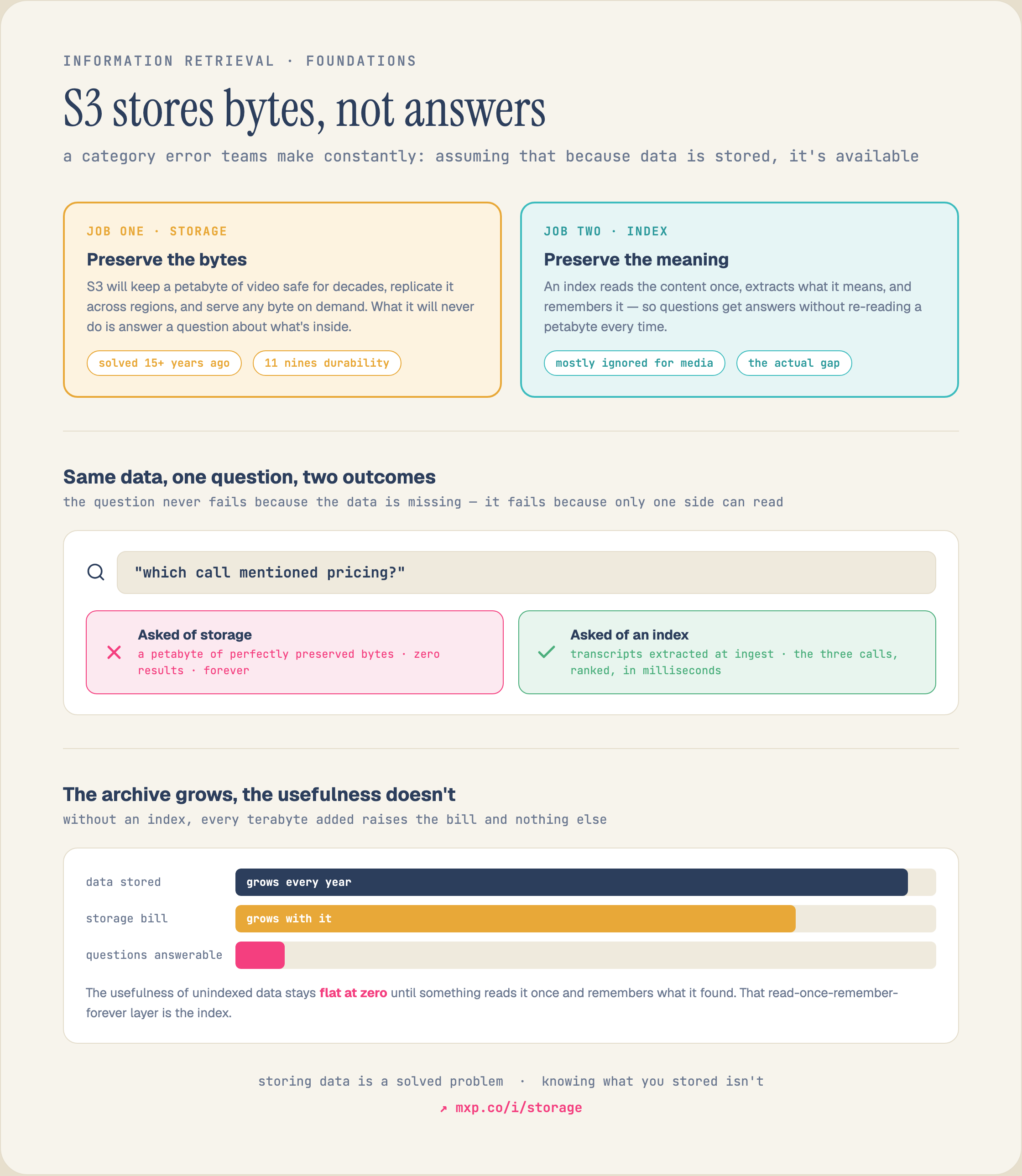
    Storage versus index: object storage like S3 preserves the raw bytes durably but can never answer a question about what is inside them, while an index reads the content once, extracts what it means, and remembers it so queries get answered in milliseconds without re-reading everything. Without an index, every added terabyte raises the storage bill while the number of answerable questions stays flat at zero.
    IR Foundations

    S3 stores bytes, not answers

    Storage keeps the bytes; an index keeps the meaning: the archive is only useful once it is indexed.
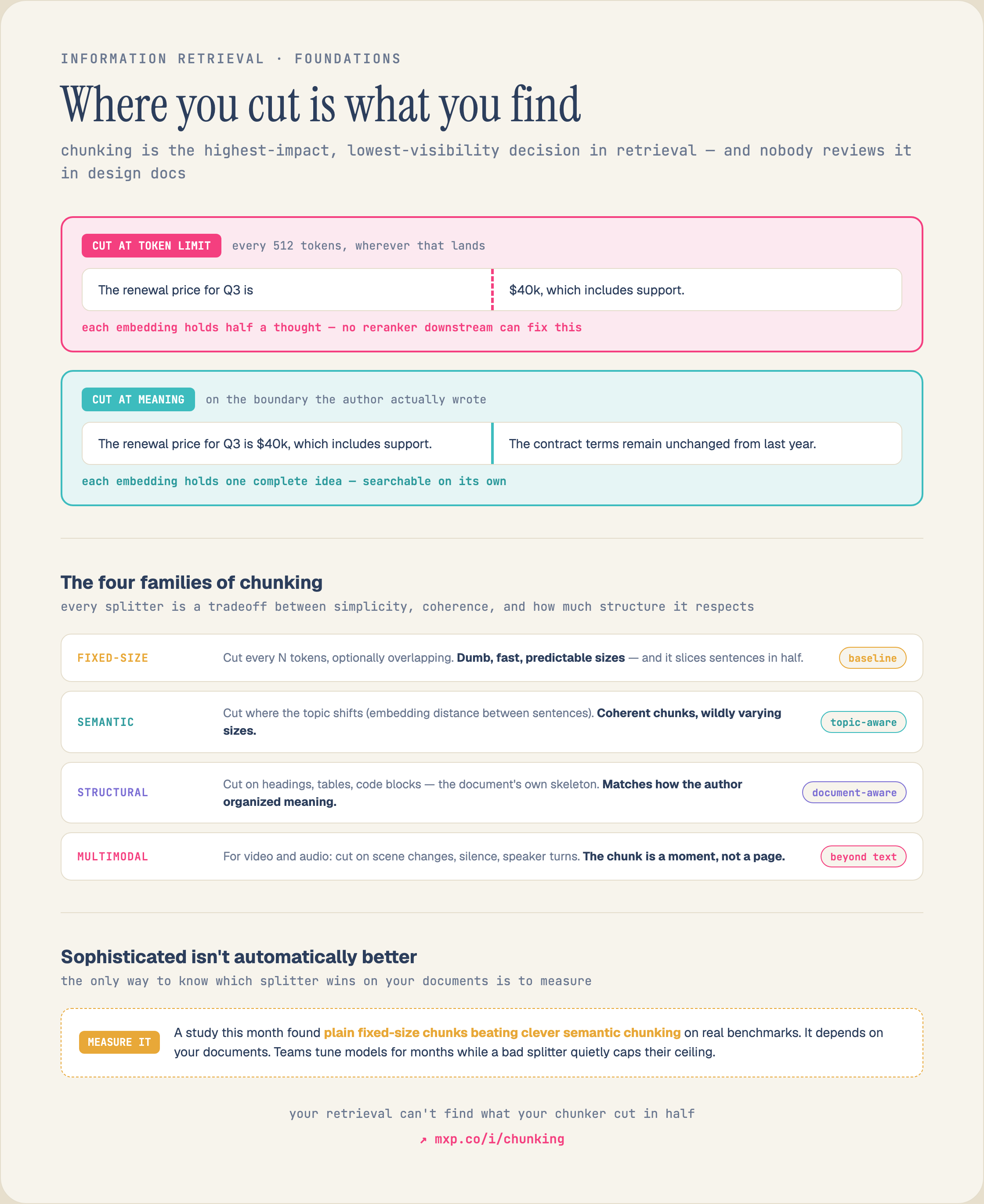
    How you split a document decides what you can find: fixed-size chunks cut mid-sentence and strand the answer across two pieces, while splitting on meaning keeps each chunk a complete thought. Chunk too small and you lose the context that makes an answer usable; chunk too large and the relevant sentence is diluted by everything around it.
    IR Foundations

    How you split decides what you find

    How you split decides what you find
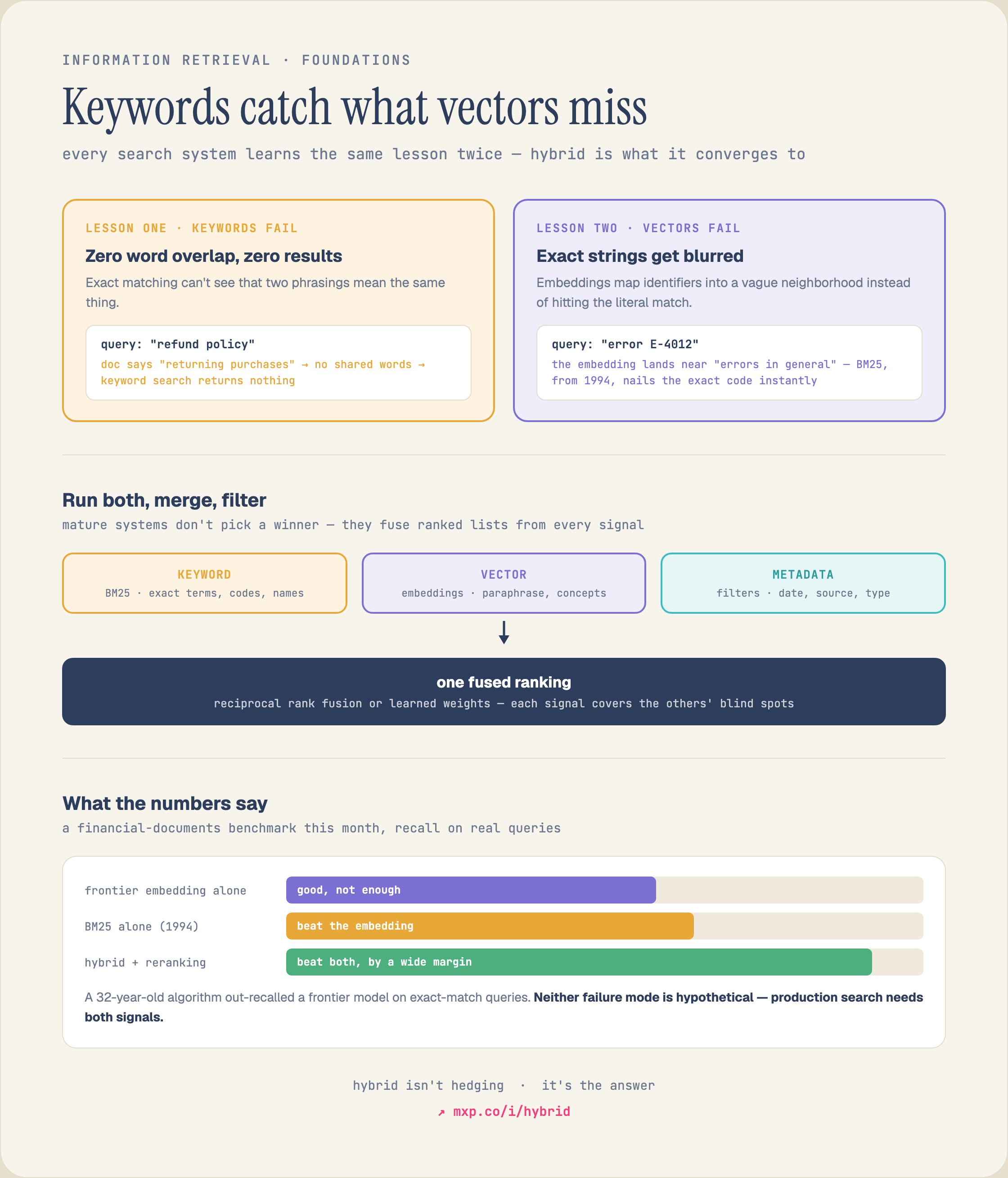
    Hybrid retrieval combines keyword and vector search because each fails alone: keyword (BM25) search misses paraphrases with zero word overlap, while dense embeddings blur exact identifiers like error codes. Mature systems run keyword, vector, and metadata signals together and fuse the ranked lists, reciprocal rank fusion or learned weights, so each signal covers the others' blind spots.
    IR Foundations

    Keywords catch what vectors miss

    Hybrid search fuses keyword (BM25) and vector results so each covers the other's blind spots.
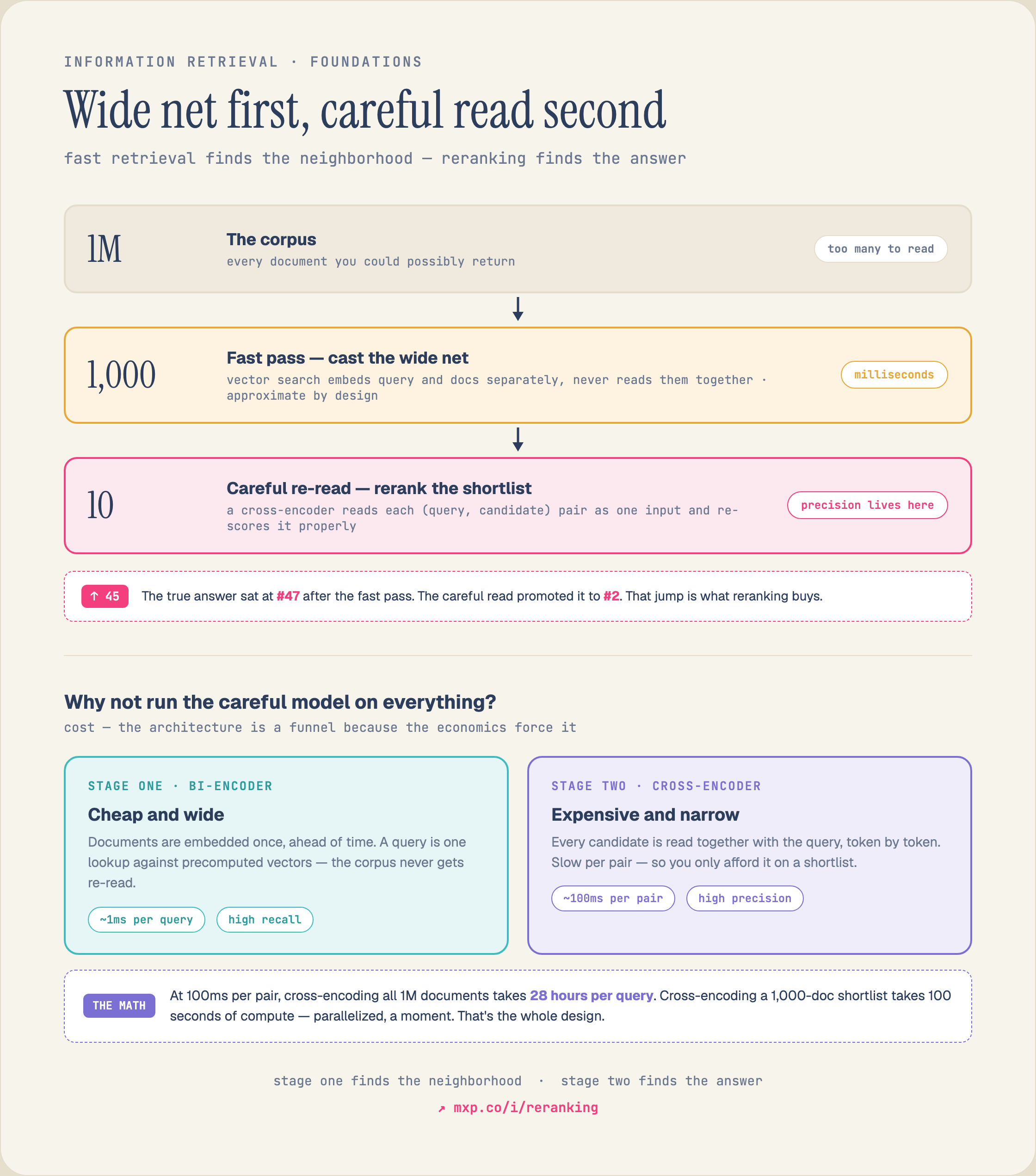
    Reranking is the precision second stage of retrieval: a fast first-stage retriever recalls a broad candidate set optimized for recall, then a cross-encoder reranker reads each query-document pair together and re-scores them so the most relevant results rise to the top before they reach the model. Fast recall first, precise scoring second.
    IR Foundations

    Wide net first, careful read second

    Reranking re-scores first-stage candidates with a cross-encoder so the best results rise to the top.
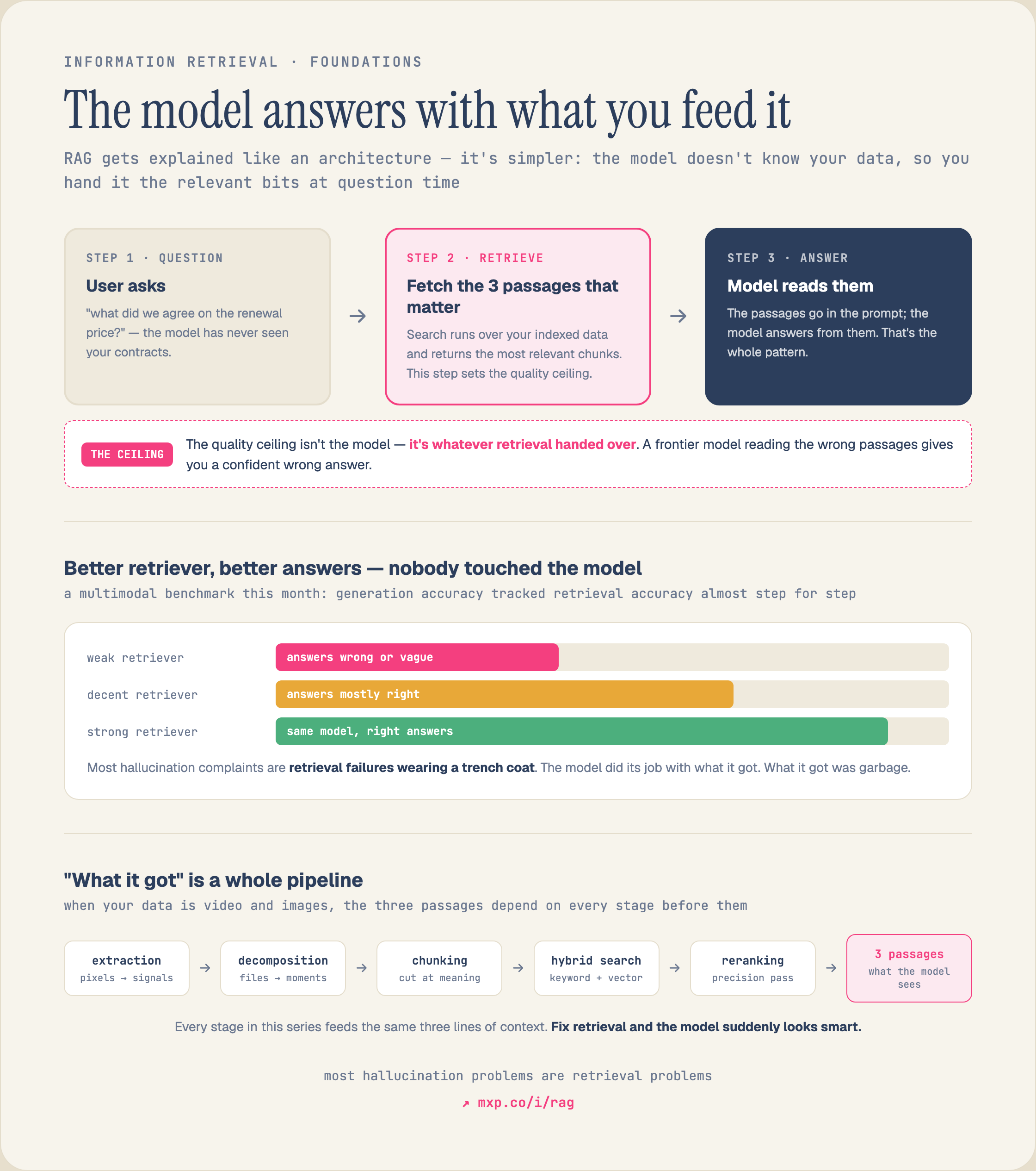
    Retrieval-augmented generation (RAG): a user asks a question, search retrieves the few most relevant passages from your indexed data, and the model answers from those passages placed in its prompt. The quality ceiling is retrieval, not the model: most hallucinations are retrieval failures, because the model can only answer with what it was fed.
    IR Foundations

    The model answers with what you feed it

    In RAG, retrieval sets the quality ceiling: the model answers from the passages you feed it.
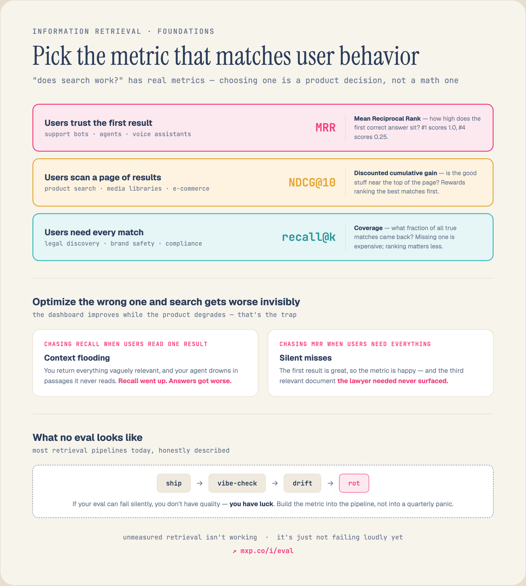
    Choosing a retrieval eval metric is a product decision, not a math one: use Mean Reciprocal Rank (MRR) when users trust the first result (support bots, agents, voice assistants), NDCG@10 when users scan a page of results (product and media search, e-commerce), and recall@k when users need every match (legal discovery, brand safety, compliance). Optimizing the wrong metric makes the dashboard improve while the product degrades, and unmeasured retrieval is not working: it is just not failing loudly yet.
    IR Foundations

    Pick the metric that matches user behavior
    Pick the metric that matches user behavior

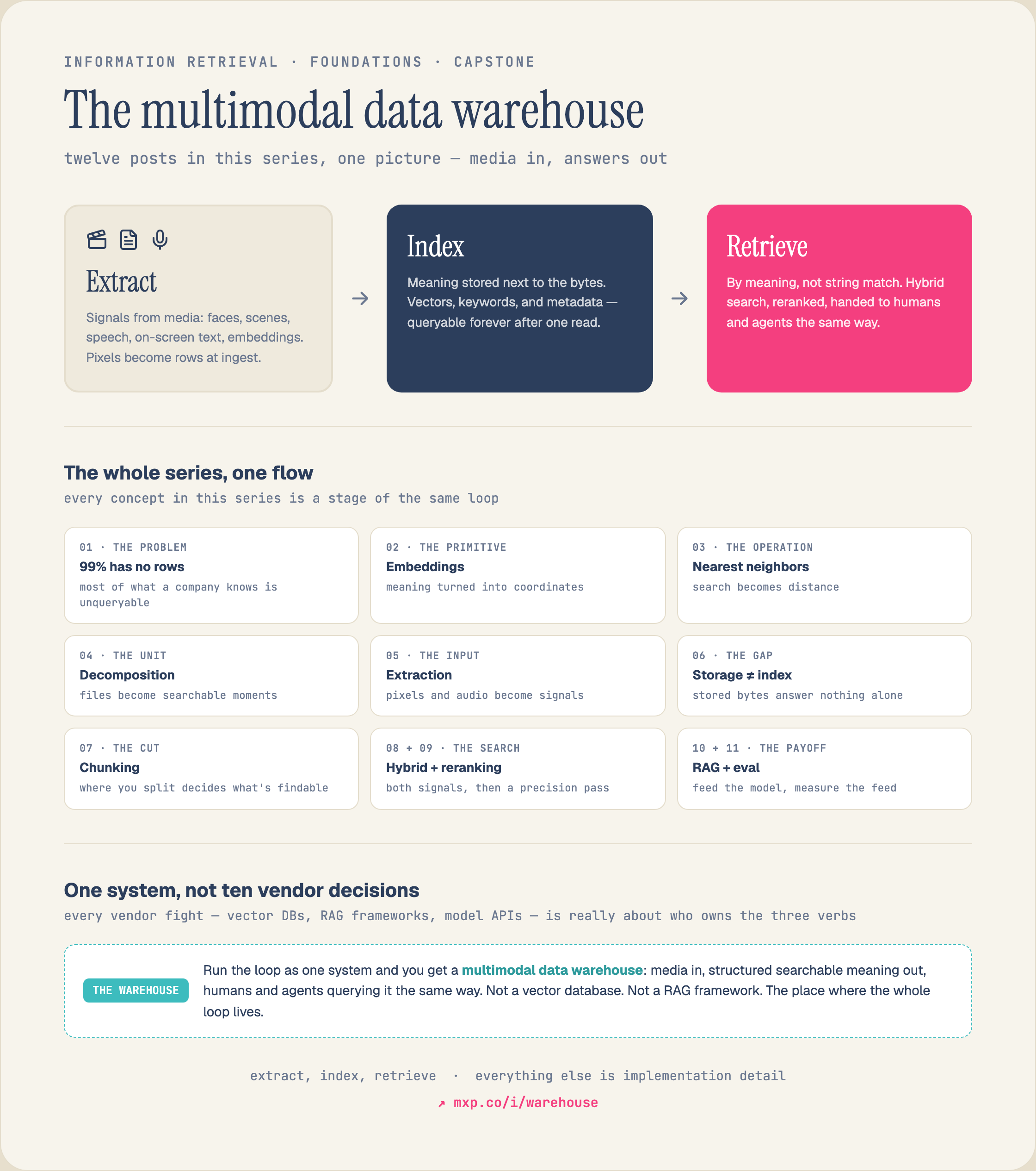
    The multimodal data warehouse in one flow: extract signals from media (faces, scenes, speech, on-screen text, embeddings) so pixels become rows at ingest, index that meaning next to the bytes so it is queryable forever after one read, and retrieve by meaning with hybrid search and reranking, served to humans and agents the same way. Extract, index, retrieve; everything else is implementation detail.
    IR Foundations

    Extract, index, retrieve: the whole loop
    Extract, index, retrieve: the whole loop

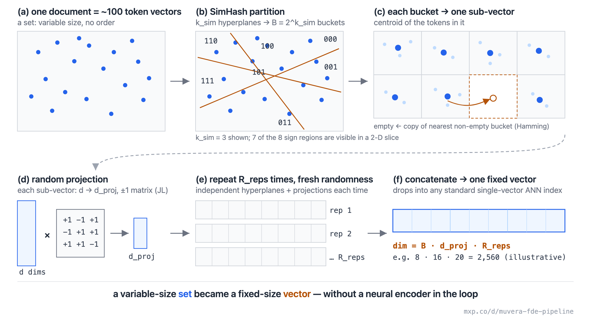
    A variable-size set of token vectors becomes one fixed-size vector via SimHash bucketing, projection, and repetition: no neural encoder required.
    MUVERA / Multi-Vector

    MUVERA: How a Multi-Vector Set Becomes One Fixed Vector

    How a Multi-Vector Set Becomes One Fixed Vector
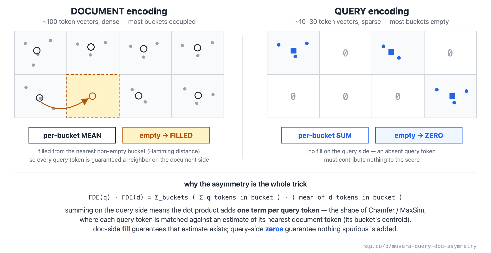
    Documents fill empty buckets with a mean; queries sum and leave empty buckets zero: the asymmetry is what makes the FDE dot product approximate Chamfer / MaxSim.
    MUVERA / Multi-Vector

    MUVERA: Why Query and Document Are Encoded Asymmetrically

    Why Query and Document Are Encoded Asymmetrically
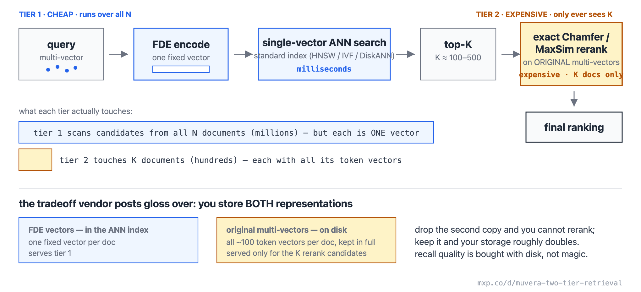
    Tier 1 FDE-encodes the query and does fast single-vector ANN over all N to get a top-K; tier 2 reranks only those K with exact Chamfer over the original token vectors.
    MUVERA / Multi-Vector

    MUVERA: Two-Tier Retrieval (Cheap FDE Recall, Exact Rerank)

    Two-Tier Retrieval (Cheap FDE Recall, Exact Rerank)
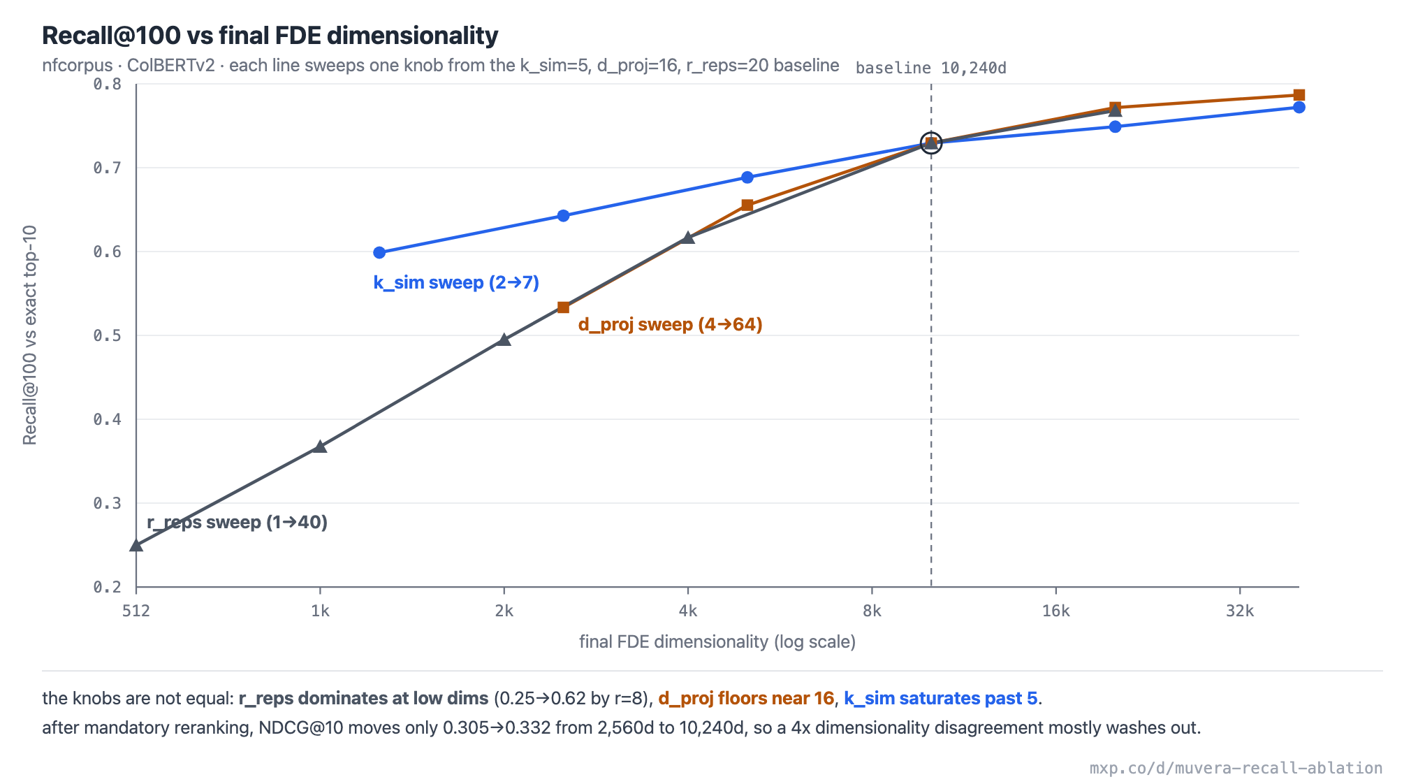
    Recall@100 versus final FDE dimensionality on nfcorpus with ColBERTv2, log x-axis, one line per swept knob (k_sim, d_proj, r_reps); r_reps dominates at low dimensionality, d_proj floors near 16, and k_sim saturates past 5.
    MUVERA / Multi-Vector

    MUVERA: Which Knob Actually Buys Recall (FDE Dimensionality Ablation)

    Which Knob Actually Buys Recall (FDE Dimensionality Ablation)
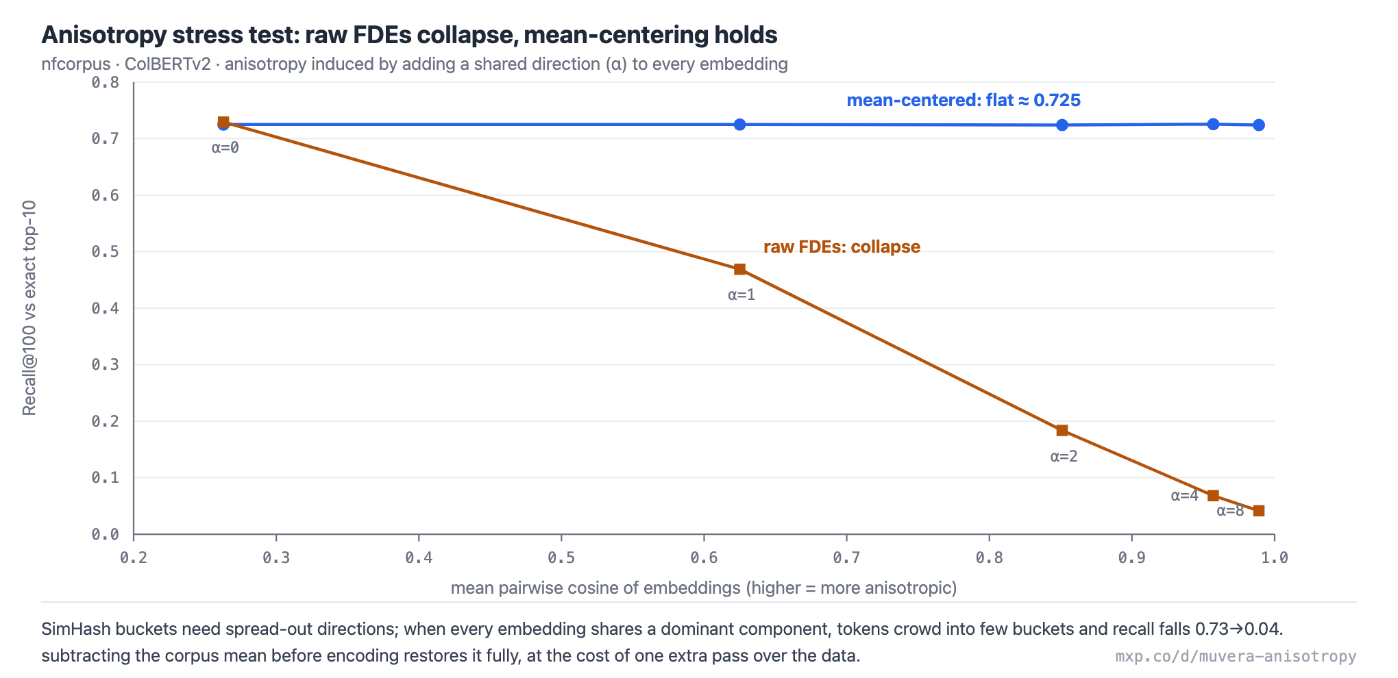
    As the mean pairwise cosine of the embeddings rises from 0.26 to 0.99, raw FDE Recall@100 collapses from 0.73 to 0.04, while the mean-centered line stays flat at about 0.725.
    MUVERA / Multi-Vector

    MUVERA: Why Anisotropic Embeddings Break FDEs (and Mean-Centering Fixes It)

    Why Anisotropic Embeddings Break FDEs (and Mean-Centering Fixes It)

    Four chunking strategies applied to the same document: fixed-size cuts mid-sentence, semantic splits on topic shifts, hierarchical nests children under retrievable parents, document-aware respects headings, code blocks, and tables.
    Diagram Series

    Four Chunking Strategies, Same Document
    Four Chunking Strategies, Same Document

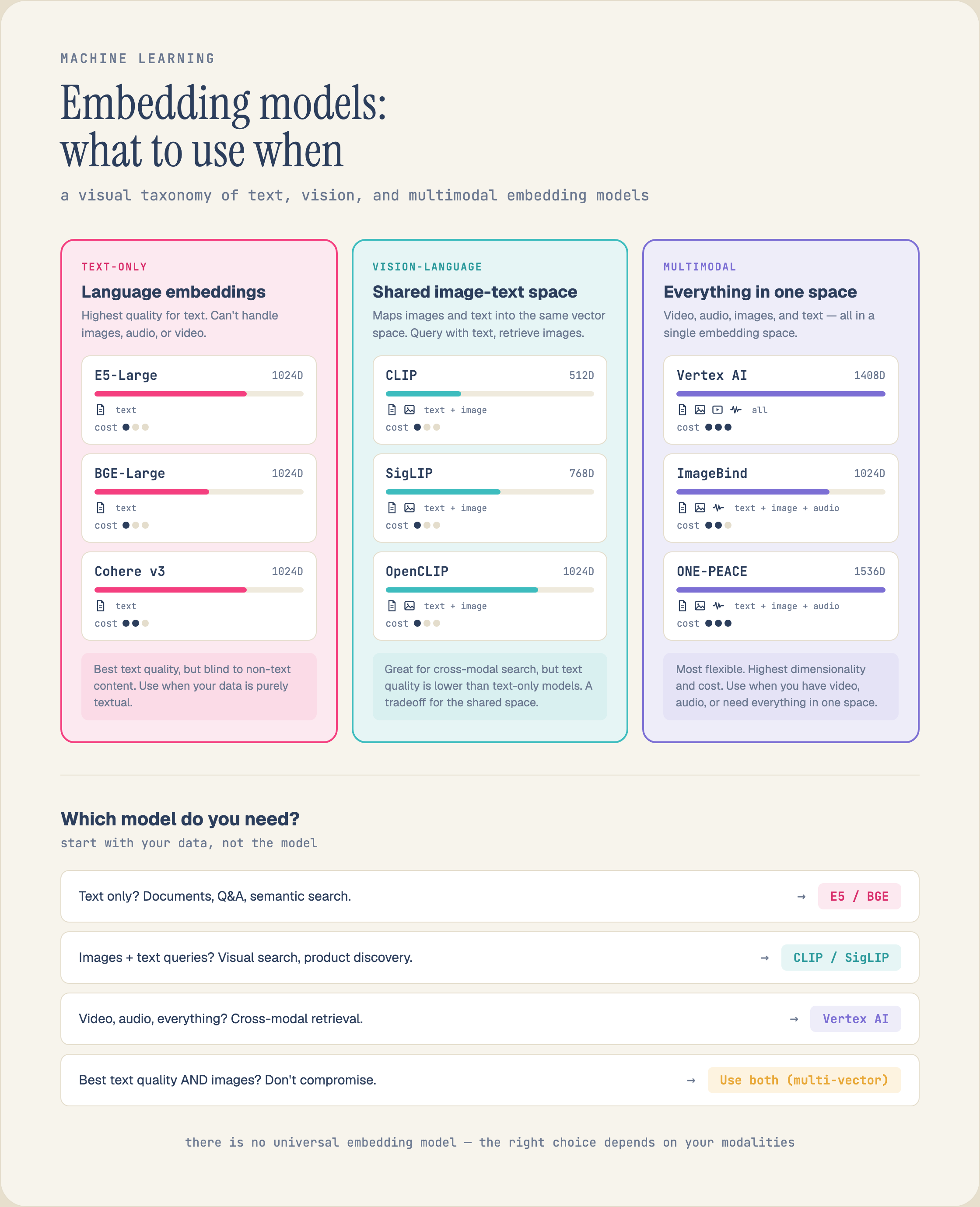
    The embedding model landscape: text-only models (E5, BGE, Cohere) for pure text, vision-language models (CLIP, SigLIP, OpenCLIP) for image plus text search, and multimodal models (Vertex 1408D, ImageBind, ONE-PEACE) when video, audio, images, and text must share one space.
    Diagram Series

    The Embedding Model Landscape

    The Embedding Model Landscape
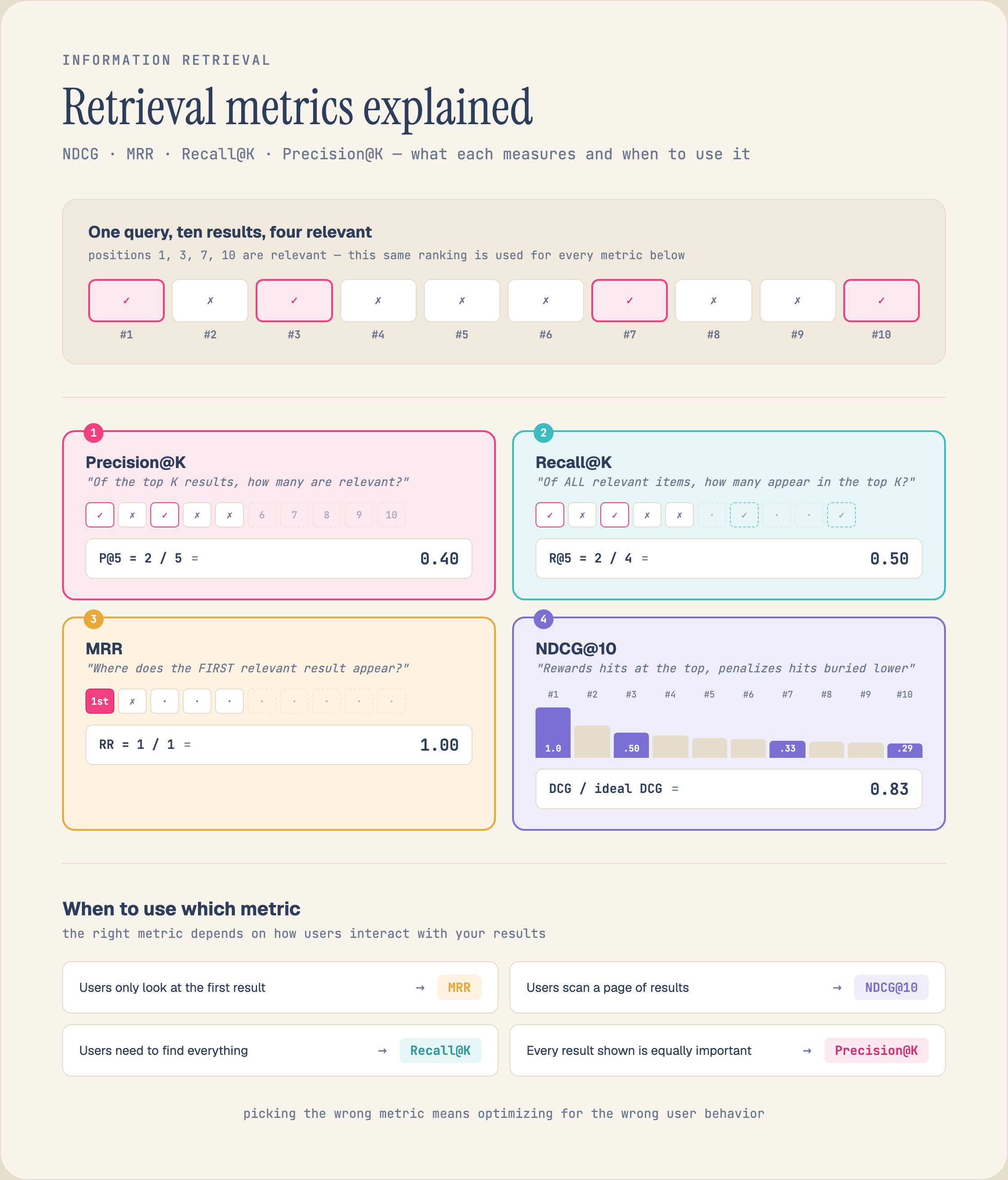
    One ranking, four metrics: with relevant results at positions 1, 3, 7, and 10, Precision@5 = 0.40, Recall@5 = 0.50, MRR = 1.0, NDCG@10 = 0.83. The right metric depends on how users read your results.
    Diagram Series

    One Ranking, Four Metrics

    One Ranking, Four Metrics
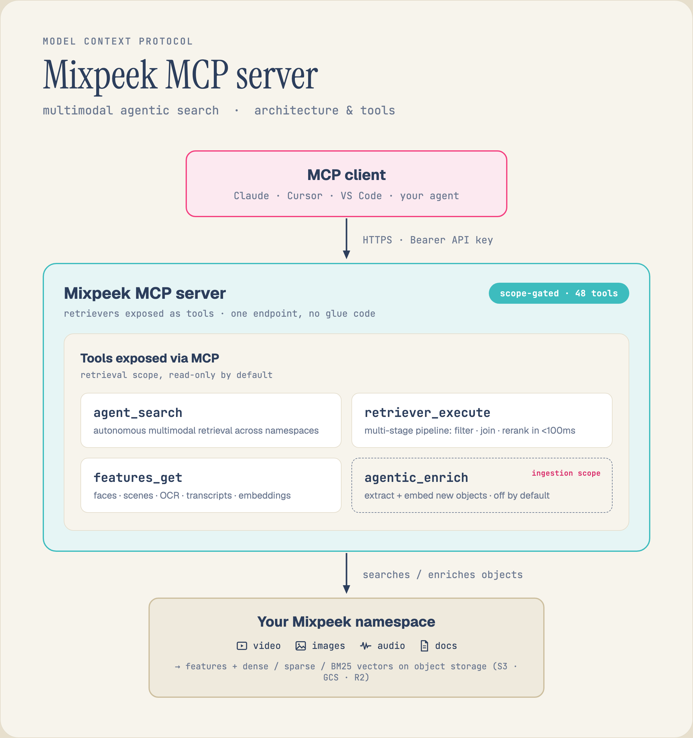
    Multimodal search exposed to an AI agent as an MCP tool: the agent calls a single search tool and Mixpeek runs retrieval across video, images, audio, and documents, returning timestamped, cited results the agent can reason over.
    Diagram Series

    Multimodal Search as an MCP Tool

    Multimodal Search as an MCP Tool

    Video highlight detection pipeline: a video is decomposed into shots and segments, each segment is scored across visual, audio, and transcript signals, contiguous high-scoring intervals merge into moments, and moments are ranked per video.
    Diagram Series

    Multimodal Decomposition: One File, Many Signals

    Multimodal Decomposition: One File, Many Signals
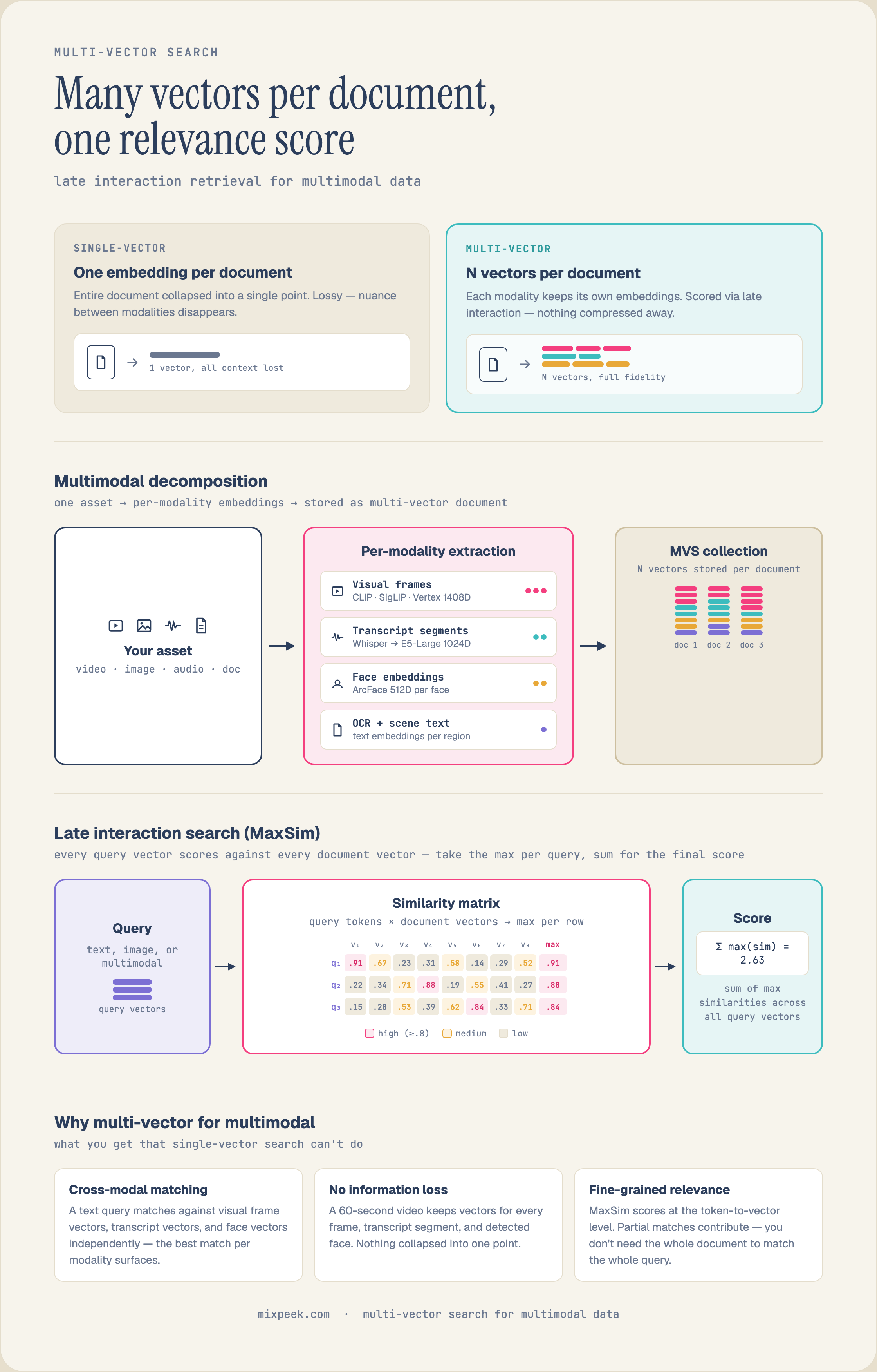
    Multi-vector (late-interaction) search versus a single embedding: instead of compressing a whole document into one vector, the model keeps one vector per token or patch and scores a query against all of them with a MaxSim operator, which recovers detail a single averaged vector loses.
    Diagram Series

    Multi-Vector Search vs. a Single Embedding
    Multi-Vector Search vs. a Single Embedding

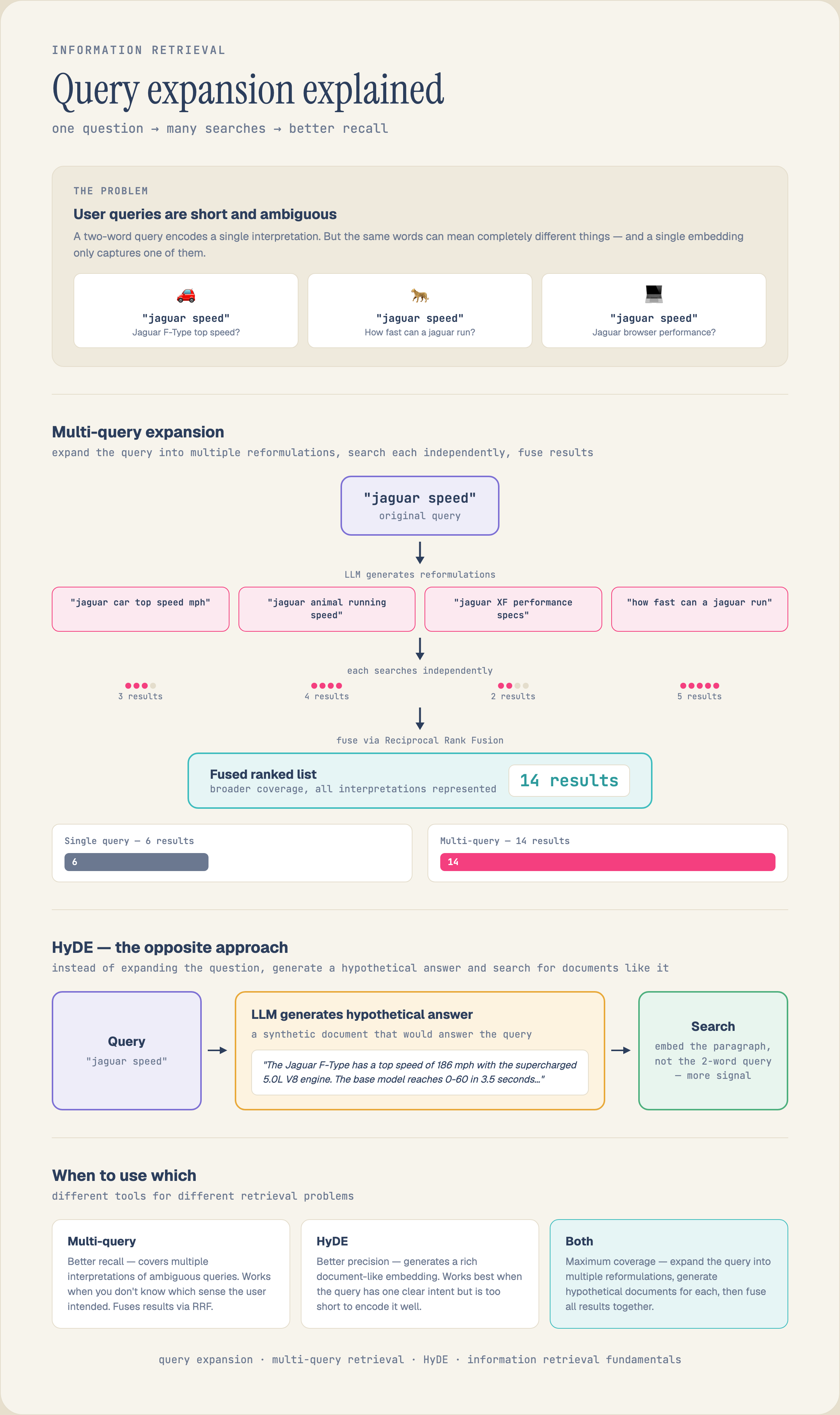
    Query expansion rewrites the user's question before retrieval: a short or ambiguous query is expanded into related terms, synonyms, and sub-questions, so first-stage search matches documents the literal phrasing would have missed.
    Diagram Series

    Query Expansion: Rewriting the Question Before You Search

    Query Expansion: Rewriting the Question Before You Search

    How reranking works: a fast bi-encoder recalls ~1,000 candidates from the full corpus, then a cross-encoder jointly scores each (query, document) pair to reorder the top results, fast recall, then precise scoring.
    Diagram Series

    How Reranking Works: Recall Wide, Then Score Precisely

    How Reranking Works: Recall Wide, Then Score Precisely
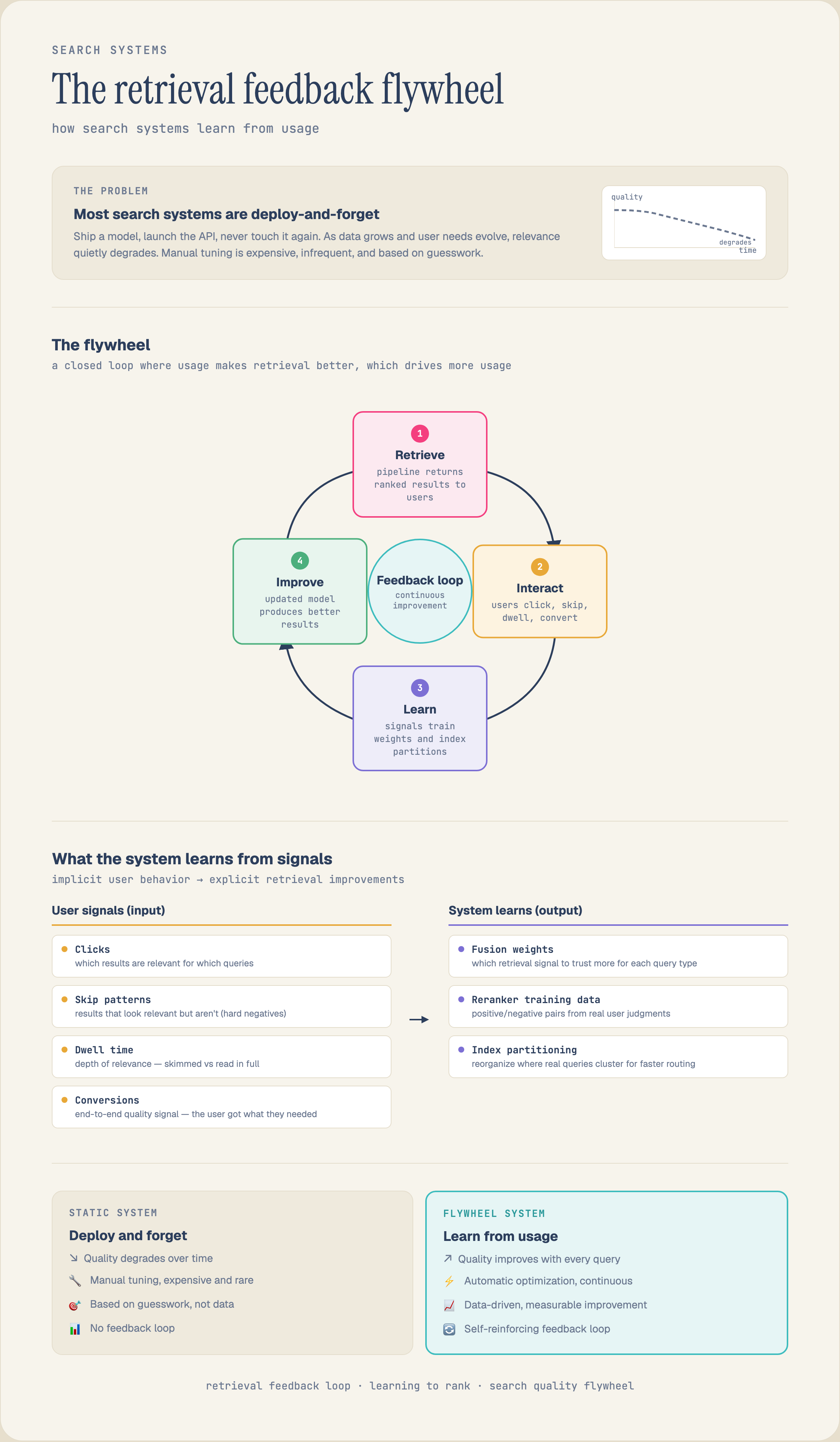
    The retrieval feedback flywheel: retrieve, interact, learn, improve, clicks, skips, dwell time, and conversions become fusion weights, reranker training pairs, and index partitioning.
    Diagram Series

    The Retrieval Feedback Flywheel

    The Retrieval Feedback Flywheel
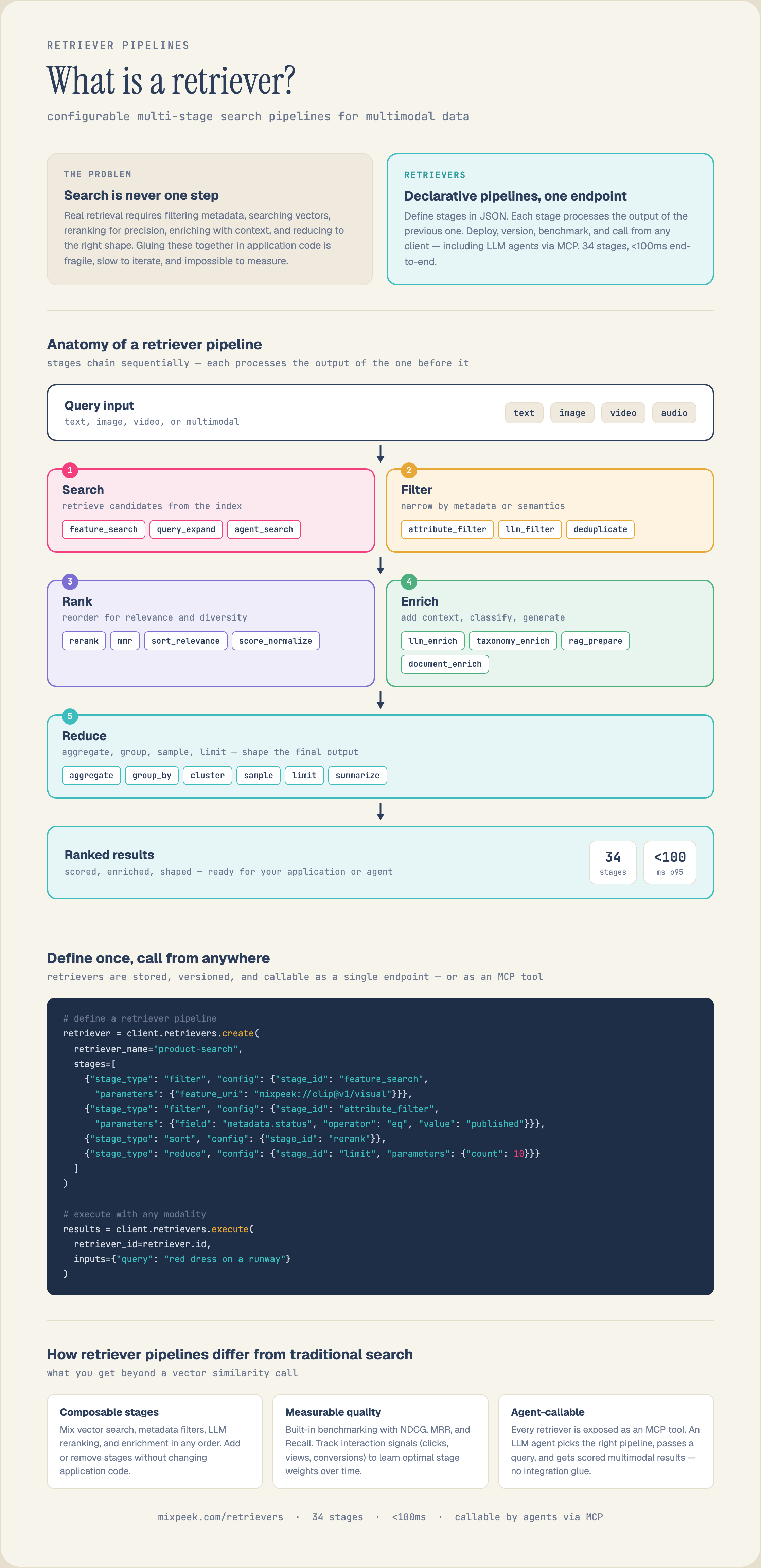
    Anatomy of a retriever pipeline: a query flows through staged operations (filtering, first-stage dense or hybrid search, then reranking) with each stage narrowing and reordering candidates before results are returned.
    Diagram Series

    Anatomy of a Retriever Pipeline

    Anatomy of a Retriever Pipeline
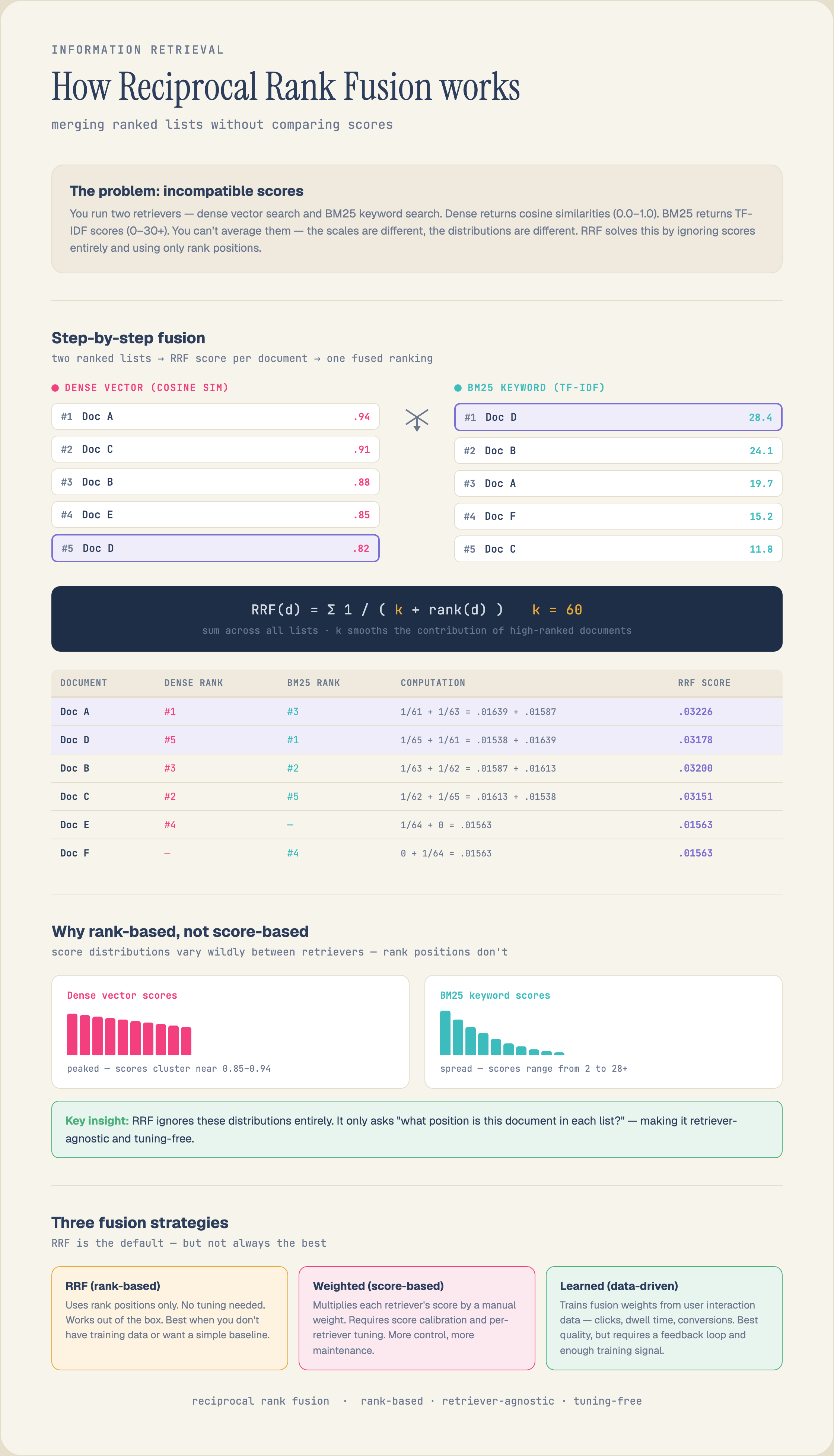
    Reciprocal Rank Fusion step by step: dense and BM25 result lists merge by rank position, RRF(d) = sum of 1/(k + rank) with k = 60, so incompatible score scales never need calibration.
    Diagram Series

    Reciprocal Rank Fusion, Explained

    Reciprocal Rank Fusion, Explained
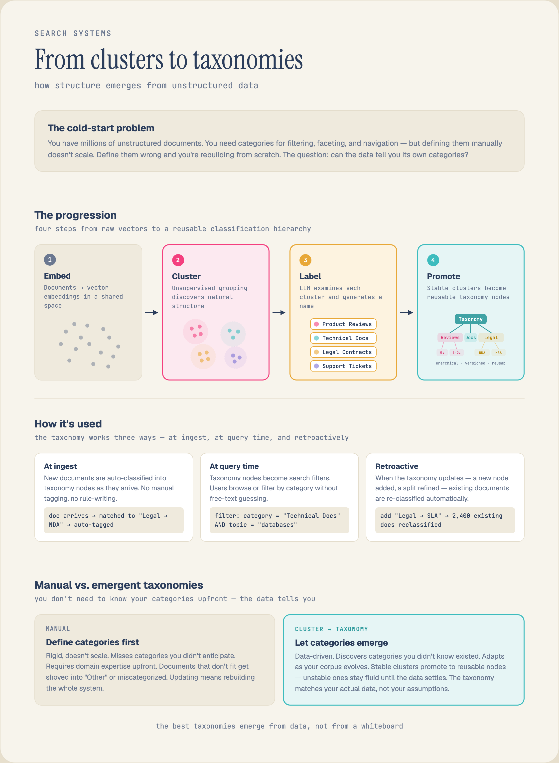
    Taxonomy-aware retrieval: documents are enriched with taxonomy labels at ingest, so a query can be scoped or boosted by category, letting search combine semantic similarity with a governed classification instead of relying on embeddings alone.
    Diagram Series

    Taxonomy-Aware Retrieval

    Taxonomy-Aware Retrieval
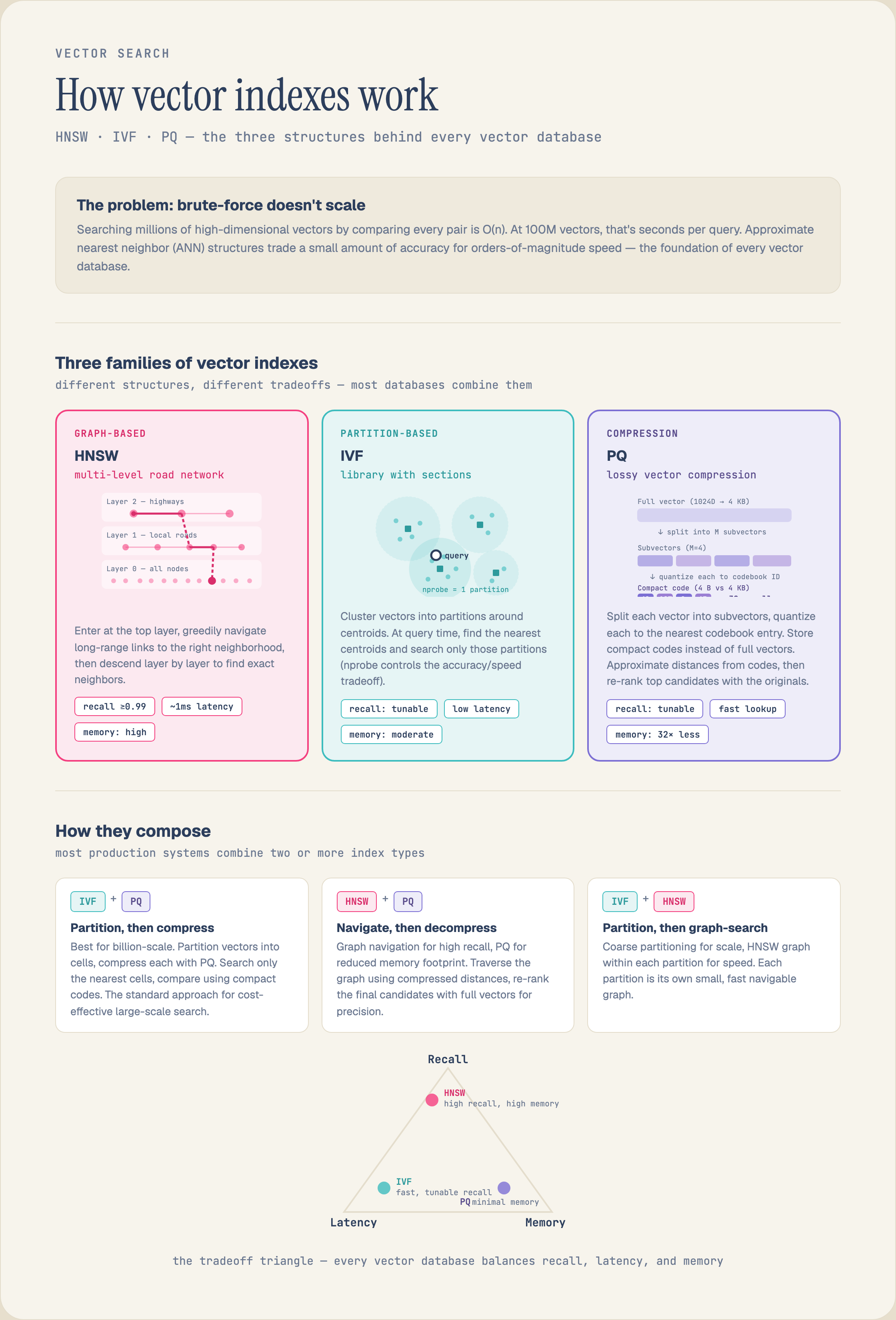
    The three structures behind every vector database: HNSW graphs navigate layered links for high recall, IVF searches only the nearest partitions, PQ compresses vectors roughly 32x, and production systems compose them.
    Diagram Series

    Vector Index Structures: HNSW, IVF, and Friends
    Vector Index Structures: HNSW, IVF, and Friends

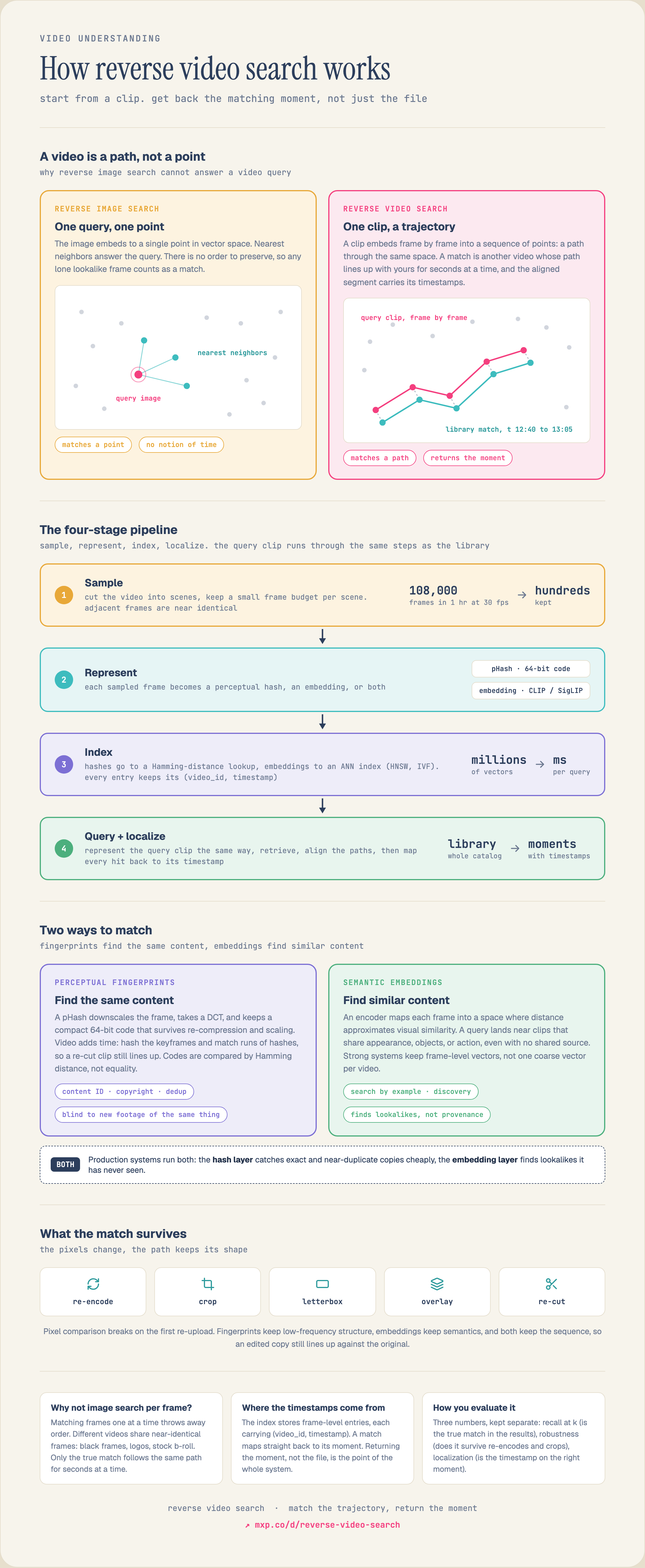
    Reverse image search embeds one image and returns nearest neighbors: it matches a point in embedding space. A video clip embeds frame by frame into a trajectory through that same space, so reverse video search means finding another video whose path lines up with yours for seconds at a time, and the aligned segment carries its timestamps. The four-stage pipeline samples frames, represents them as perceptual fingerprints or semantic embeddings, indexes them with (video_id, timestamp) payloads, and localizes the matching moment. The match survives re-encodes, crops, letterboxing, overlays, and re-cuts because the pixels change but the path keeps its shape.
    Video Retrieval

    Reverse Video Search: A Clip Is a Trajectory, Not a Point

    Why image reverse-search matches a point and video reverse-search matches a path.
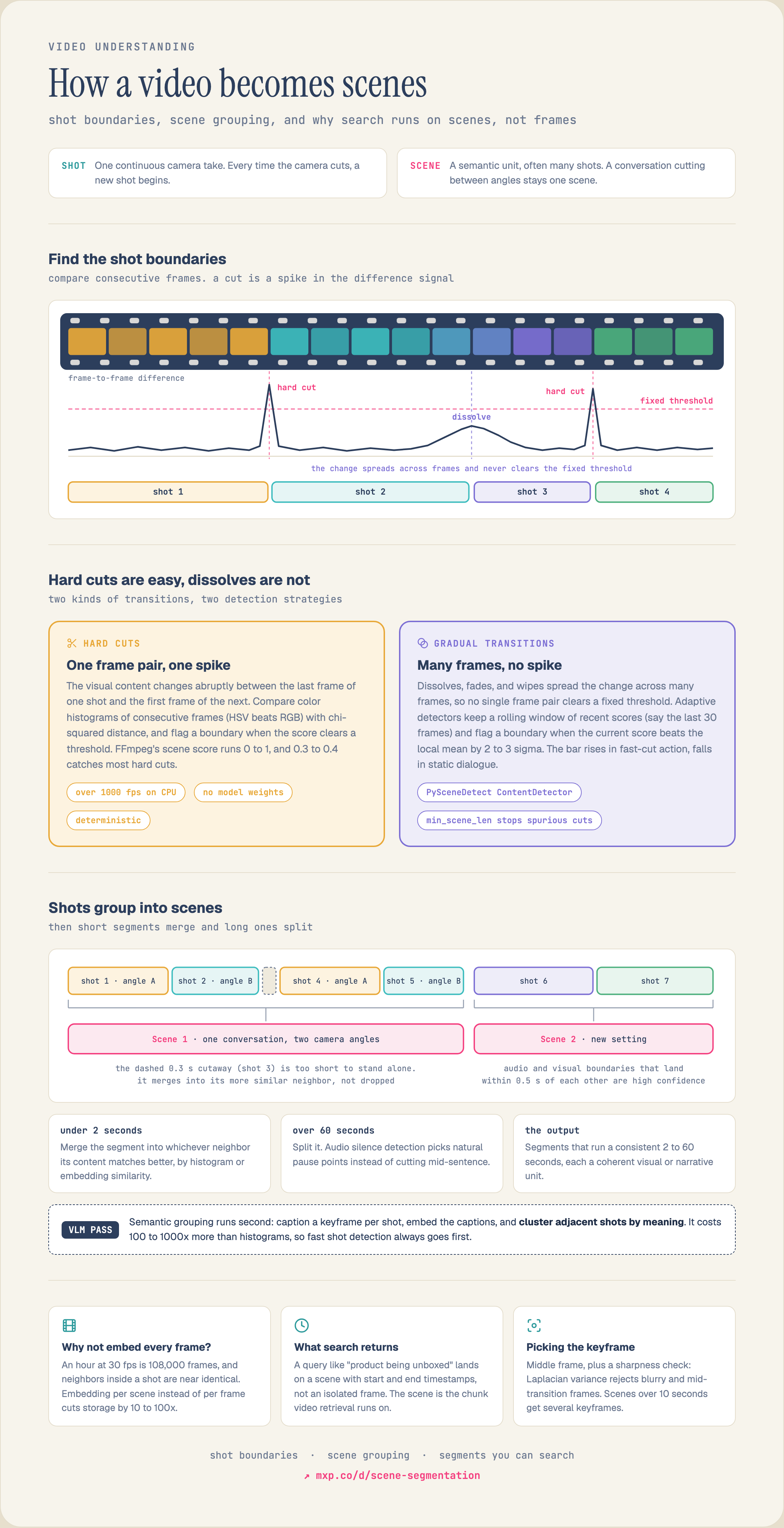
    Scene segmentation turns a continuous video into searchable segments in two levels. First, shot boundary detection compares consecutive frames: a hard cut spikes a histogram difference (over 1000 fps on CPU), while dissolves and fades spread the change across many frames, so adaptive detectors flag a boundary when the score beats a rolling local mean by 2 to 3 sigma. Second, shots group into scenes, where a shot is one continuous camera take and a scene is a semantic unit that can span many shots. Cleanup rules merge segments under 2 seconds into their nearest neighbor and split segments over 60 seconds at audio silence. The scene becomes the retrieval unit: one embedding per scene instead of per frame, results that carry start and end timestamps, and storage down 10 to 100x.
    Video Understanding

    Scene Segmentation: How a Video Becomes Searchable Scenes

    A raw video has no scenes. Two levels of boundary detection turn 108,000 frames an hour into a handful of searchable segments.
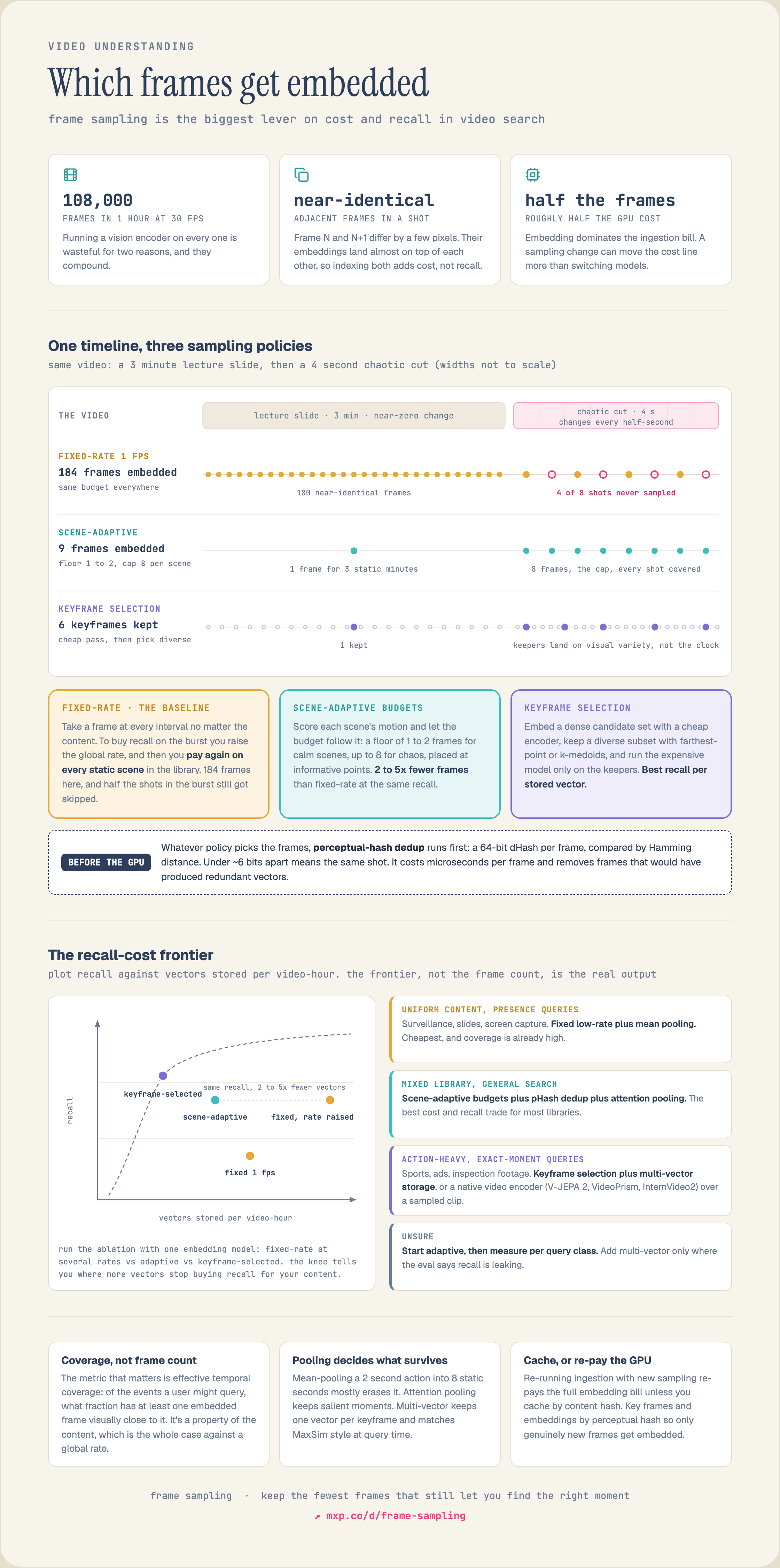
    Frame sampling decides which frames of a video get embedded, the single biggest lever on cost and recall. An hour of 30 fps video is 108,000 frames, and adjacent frames within a shot are near identical, so their embeddings land almost on top of each other and indexing both adds storage and query fan-out, not recall. The same timeline (a 3 minute lecture slide, then a 4 second chaotic cut) sampled three ways: fixed rate 1 fps embeds 184 frames and still skips half the shots in the burst, a scene-adaptive budget covers everything with 9, and embedding-space keyframe selection keeps 6 chosen for visual diversity. The real output is the recall versus cost frontier: plot recall against vectors stored per video-hour and find the knee for your content, per query class.
    Video Understanding

    Frame Sampling: Which Frames Get Embedded, and What It Costs

    Embedding is the expensive step, so the frames you choose to embed are the biggest lever on the cost and recall of a video search system.
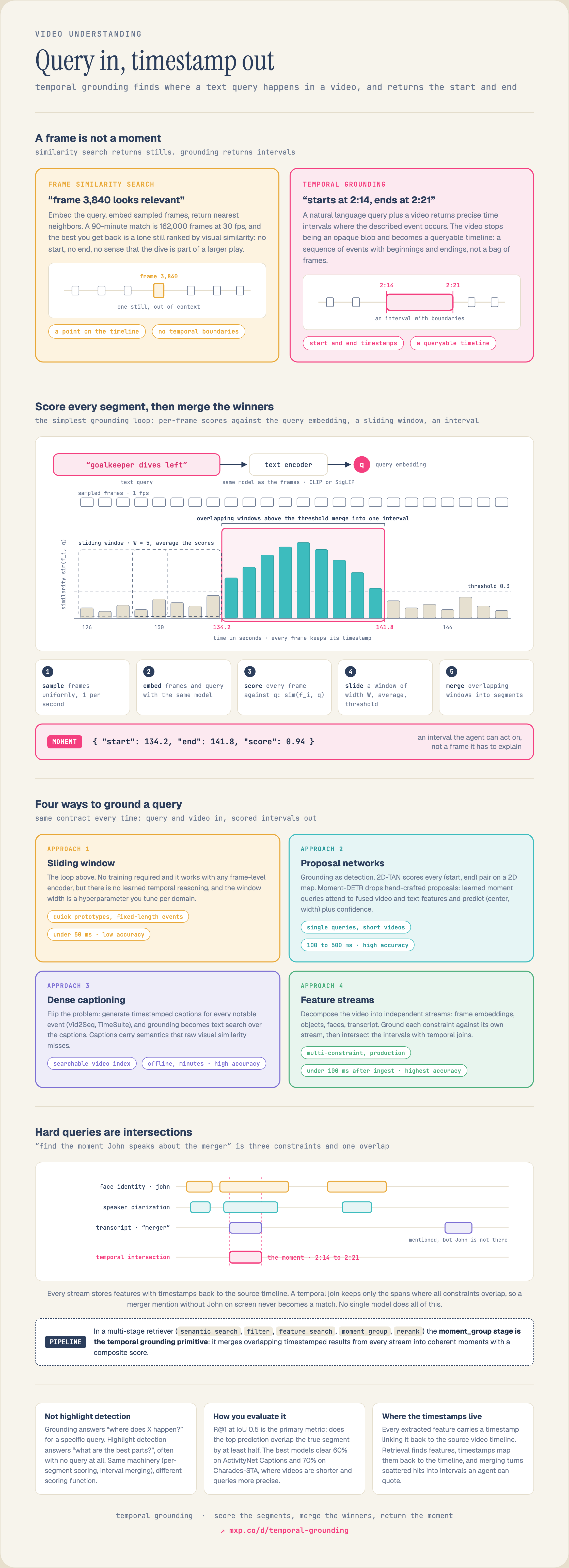
    Temporal grounding takes a natural language query and a video and returns the start and end timestamps of the described event, turning the video from an opaque blob into a queryable timeline. Frame-level similarity search only returns stills: the best it can say is that one frame looks relevant, with no beginning or end. The core loop is per-segment scoring plus interval merging: sample frames at 1 fps, embed frames and query with the same model (CLIP or SigLIP), score every frame against the query, slide a window and average the scores, then merge the overlapping windows that clear a threshold into one segment with a start and an end (for example start 134.2, end 141.8, score 0.94). Fancier methods keep the same contract: proposal networks like 2D-TAN and Moment-DETR learn the boundaries, dense captioning turns grounding into text search, and production systems decompose the video into timestamped feature streams and intersect intervals with temporal joins. The primary metric is Recall at 1 with IoU 0.5.
    Video Understanding

    Temporal Grounding: Query In, Timestamp Out

    Frame search returns stills. Temporal grounding takes a text query and a video and returns the start and end timestamps of the moment you asked for.
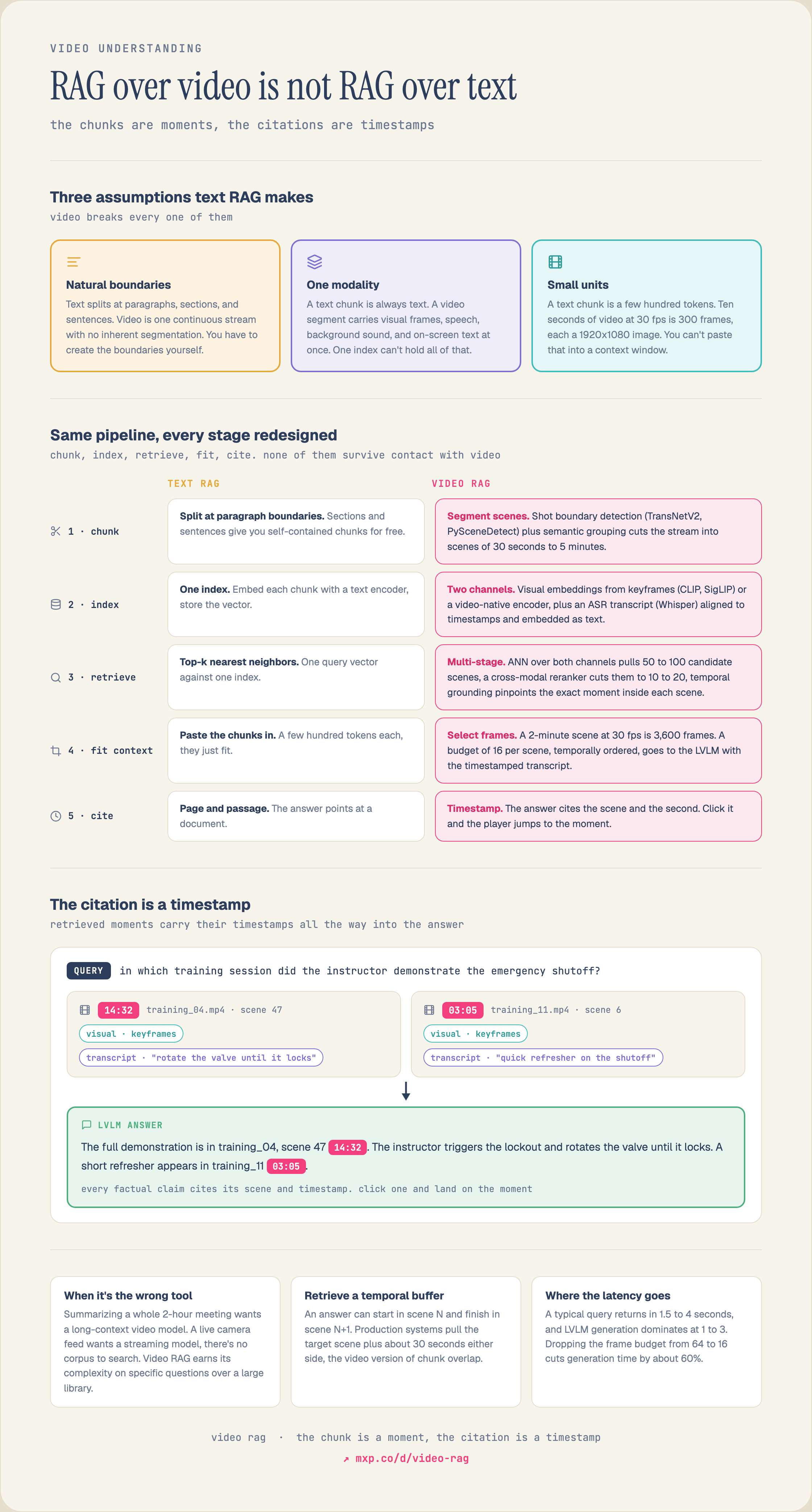
    Video RAG redesigns every stage of retrieval-augmented generation because video breaks the three assumptions text RAG relies on: natural chunk boundaries (paragraphs), a uniform modality (a chunk is always text), and small retrieval units (a few hundred tokens). Video is a continuous stream with no inherent segmentation, a single segment carries frames, speech, background sound, and on-screen text at once, and ten seconds at 30 fps is already 300 frames. So chunking becomes scene segmentation (TransNetV2, PySceneDetect, scene chunks of 30 seconds to 5 minutes), one index becomes dual-channel indexing (visual embeddings from keyframes plus a Whisper transcript aligned to timestamps), retrieval becomes multi-stage (ANN pulls 50 to 100 candidates, cross-modal reranking cuts to 10 to 20, temporal grounding pinpoints the moment), context assembly becomes frame selection (about 16 frames per scene, temporally ordered, diminishing returns past 32 to 64), and the citation becomes a timestamp the user can click to land on the exact moment.
    Video Understanding

    Video RAG: Why Retrieval Over Video Is Not Retrieval Over Text

    Text RAG gets chunk boundaries, one modality, and small units for free. Video gives you none of them, so every stage of the pipeline is redesigned.

    Speaker diarization answers who spoke and when, the layer transcription alone cannot provide. The same sixteen seconds of a meeting are shown at three levels: the raw waveform, voice activity detection marking speech regions, and clustered speaker turns, producing a transcript whose every line carries a speaker label and a timestamp. The standard pipeline is four stages: voice activity detection (Silero VAD, a 2MB model running 500x real-time on CPU at about 95% accuracy), speaker embedding extraction (ECAPA-TDNN, 192 or 256 dimensions over 1.5 to 3 second sliding windows, capturing pitch and timbre regardless of words), spectral clustering that reads the speaker count from the eigenvalue gap, and overlap detection that allows multiple labels on one region. Diarization is then joined with ASR word timestamps to attribute each word, and the field scores itself with diarization error rate (false alarm plus missed speech plus speaker confusion over total speech), where under 10% is production quality.
    Video Understanding

    Speaker Diarization: Who Said What, and When

    Transcription tells you what was said. Diarization tells you who said it and when, by clustering voices before it ever aligns them to the transcript.
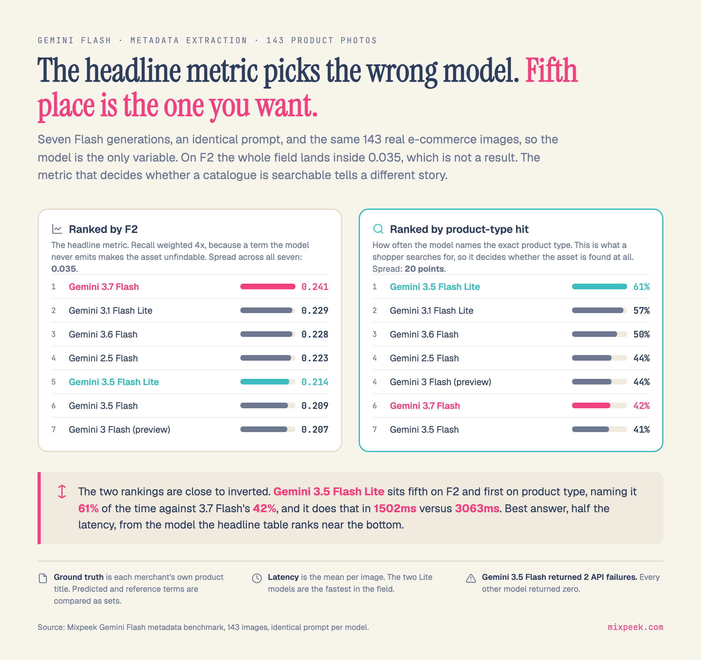
    Two rankings of seven Gemini Flash generations on metadata extraction over 143 product photos, close to inverted. Ranked by F2: 3.7 Flash 0.241, 3.1 Flash Lite 0.229, 3.6 Flash 0.228, 2.5 Flash 0.223, 3.5 Flash Lite 0.214, 3.5 Flash 0.209, 3 Flash preview 0.207, a spread of 0.035. Ranked by how often the model names the exact product type: 3.5 Flash Lite 61 percent, 3.1 Flash Lite 57, 3.6 Flash 50, 2.5 Flash 44, 3 Flash preview 44, 3.7 Flash 42, 3.5 Flash 41, a spread of 20 points. Gemini 3.5 Flash Lite sits fifth on F2 and first on product type, at 1502ms against 3.7 Flash's 3063ms.
    Benchmarks

    Gemini Flash Metadata Extraction: The Headline Metric Picks the Wrong Model

    Seven Gemini Flash generations, one prompt, 143 real product photos. The F2 spread is 0.035, so the headline ranking is noise. The model that names the exact product type most often is fifth in it.

    A portrait diagram in two rails. The headline reads Filters exclude, what ranking would have shown, with the subline: a pre_filter drops rows before ranking is ever shown to you, useful, and it hides what it removed. A search bar holds the query yellow armchair, annotated: three of the top five are out of stock. Rail A, badged no filter, shows five armchair photos in rank order with prices and scores: 872 dollars at 0.080, 515 dollars at 0.065, 180 dollars at 0.060, 451 dollars at 0.060 and 506 dollars at 0.057; the second, third and fourth are greyed and stamped dropped, and the count chip reads 5 of 5. Rail B, badged pre_filter with in_stock equals true, shows the two survivors at 872 and 506 dollars followed by three new armchairs at 123 dollars 0.048, 446 dollars 0.047 and 606 dollars 0.046; its chip reads 2 kept plus 3 new. A bold line states that three of the top five were out of stock and all three were removed from the response entirely. A dark code window shows the execute request with the filters line in_stock true highlighted, and skip_cache true. The footer prints mxp.co/d/filters-exclude and the words real query, real ranking, mixpeek.
    Retrieval Mechanics

    Filters Exclude What Ranking Would Have Shown

    Same query, same embeddings, one filter. Three of the top five yellow armchairs were out of stock; the in_stock pre_filter removed all three from the response and three deeper matches moved up.

    A portrait diagram in two rails. The headline reads Scope decides, what can be found at all, with the subline: the same question, asked of the whole catalog and then of one category. The search bar holds the query something to keep me warm outside, annotated: the query names no category. Rail A, badged whole catalog with the note semantic reach across every category, shows five photos in rank order: a lit tent at night for 543 dollars at 0.062, a snowy forest scene for 564 dollars at 0.060, a steaming pot on a stove for 444 dollars at 0.059, boots on a textured rug for 203 dollars at 0.052, and a tent under a starry sky for 100 dollars at 0.048; the second, third and fourth are greyed and stamped dropped, and the chip reads 5 of 5. Rail B, badged scoped with category equals tent and the note only one category can answer, shows the two surviving tents followed by three more tents at 592 dollars 0.046, 73 dollars 0.039 and 554 dollars 0.029; its chip reads 2 kept plus 3 new. A bold line states that unscoped, the index answered with tents, backpacks, rugs and pans, and that scope is a decision about what is allowed to be right. A code window shows the execute request with the filters line category tent highlighted. The footer prints mxp.co/d/scope-changes-candidates.
    Retrieval Mechanics

    Scope Decides What Can Be Found at All

    Asked of the whole catalog, "something to keep me warm outside" returned a tent, a backpack, a cast iron pan, a rug and another tent. Scoped to category = tent, only tents can answer, and the ranking inside the scope is unchanged.

    A portrait diagram in two rails. The headline reads A price ceiling, is not a price sort, with the subline: a price ceiling removes the expensive matches, it does not promote the cheap ones by price. The search bar holds the query premium floor lamp, annotated: premium is a word, not a number. Rail A, badged no ceiling with the note best matches, any price, shows five photos in rank order: floor lamps at 729 dollars 0.097, 299 dollars 0.093, 908 dollars 0.092 and 322 dollars 0.089, then an armchair at 451 dollars 0.086; four are greyed and stamped dropped, only the 299 dollar lamp survives, and the chip reads 5 of 5. Rail B, badged pre_filter with price less than 300 and the note best matches under the ceiling, shows the 299 dollar lamp first at 0.093, then lamps at 230 dollars 0.071, 104 dollars 0.068, 129 dollars 0.063 and 38 dollars 0.059; its chip reads 1 kept plus 4 new. A bold line states that rank order inside the filter is still semantic, so the cheapest item lands fourth. A code window shows the execute request with the filters line price lt 300 highlighted. The footer prints mxp.co/d/numeric-filter-reranks.
    Retrieval Mechanics

    A Price Ceiling Cuts the Set and Leaves the Order Semantic

    premium floor lamp with price < 300: four of the top five are removed, and the survivors stay in similarity order. The cheapest lamp in the filtered set lands last, at $38.

    A portrait diagram in two rails. The headline reads One index, two ways to ask, with the subline: one index, one collection, two query modalities, the answers disagree. The search bar holds worn leather armchair, annotated: same corpus, same embeddings. Rail A, badged text query with the note text query against image embeddings, shows five leather armchair photos in rank order at 496 dollars 0.114, 938 dollars 0.106, 489 dollars 0.103, 606 dollars 0.097 and 872 dollars 0.085, chip 5 of 5. Rail B, badged image query with input_mode equals content and the note an image as the query itself, shows five different photos: a white wooden armchair at 446 dollars scoring 1.000, an armchair draped with a blanket at 180 dollars 0.865, a grey chair among plants at 205 dollars 0.834, a pink sofa beside a floor lamp at 104 dollars 0.824, and a grey wooden armchair at 924 dollars 0.824; its chip reads a different five. A bold line states that the image query scores 1.0 on itself, then returns a floor lamp among the armchairs, and that visual similarity answers with pixels while your taxonomy is nowhere in the embedding. A code window shows the execute request with two highlighted input lines, query worn leather armchair for rail A and image_url pointing at a Pexels photo for rail B. The footer prints mxp.co/d/text-vs-image-query.
    Retrieval Mechanics

    One Index, Two Ways to Ask: Text Query and Image Query Disagree

    Text query "worn leather armchair" against image embeddings scores 0.08 to 0.11 and returns armchairs. The same index queried with a photograph scores 1.0 on itself, then 0.86, 0.83, and puts a floor lamp at rank four.

    A portrait diagram in two rails. The headline reads The query is, the biggest knob, with the subline: no configuration changed between these two rails, only the sentence did. The search bar holds the word chair, annotated: nothing else was changed. Rail A, badged broad with the note one word, shows five modern chairs in rank order at 872 dollars 0.098, 515 dollars 0.089, 924 dollars 0.088, 180 dollars 0.087 and 446 dollars 0.087, chip 5 of 5. Rail B, badged specific with the query worn leather armchair, bright room and the note a described scene, shows five different photos: worn leather armchairs at 496 dollars 0.072, 938 dollars 0.071 and 489 dollars 0.069, a red velvet armchair in a bright interior at 451 dollars 0.067, and a dark textured armchair at 606 dollars 0.063; its chip reads a different five. A bold line states that your biggest retrieval knob is the query itself. A code window shows the execute request with two highlighted inputs lines, query chair for A and query worn leather armchair, bright room for B, then filters null and skip_cache true. The footer prints mxp.co/d/query-specificity.
    Retrieval Mechanics

    The Query Is the Biggest Knob

    "chair" and "worn leather armchair, bright room" against the same 118 image index, same retriever, no filters. Zero overlap between the two top fives. Nothing in the configuration changed.

    A portrait diagram. The headline reads Search ignores, under 400 dollars, with the subline: an embedding has no idea what a budget is, so the agent picked a second stage and wrote the filter itself. A search bar holds the query I need to furnish a reading nook under 400 dollars, annotated: 3 of 5 results break the budget. A rail badged plain search, feature_search only, semantic match with no notion of price, shows five price cards: 922 dollars Steel Floor Lamp, 451 dollars Velvet Armchair and 663 dollars Leather Armchair outlined in rose as over budget, then 180 dollars Leather Armchair and 38 dollars Wood Floor Lamp; the chip reads 3 over budget. A bold line says the agent was given the same query and the whole stage catalog as tools. Two numbered trajectory cards follow: 1, feature_search with query furniture for reading nook, 18712 ms, 5 docs; 2, attribute_filter with price lt 400, 7 ms, 1 doc. A dark result band shows 180 dollars, Leather Armchair, the one result inside the budget, and the note that it derived price less than 400 from the sentence and nobody configured a filter. A footer line reads model gemini-2.5-flash-lite, 3 iterations, confidence 0.8, cost 0.00061 dollars, then mxp.co/d/search-that-reasons and real query, real trajectory, mixpeek.
    Agentic Retrieval

    Search Ignores "Under 400 Dollars": The Agent Wrote the Filter Itself

    "I need to furnish a reading nook under 400 dollars": plain vector search returns 3 of 5 results over budget. Given the stage catalog as tools, the agent ran feature_search, then reached for attribute_filter and wrote price lt 400 itself. One result, $180, for $0.00061.
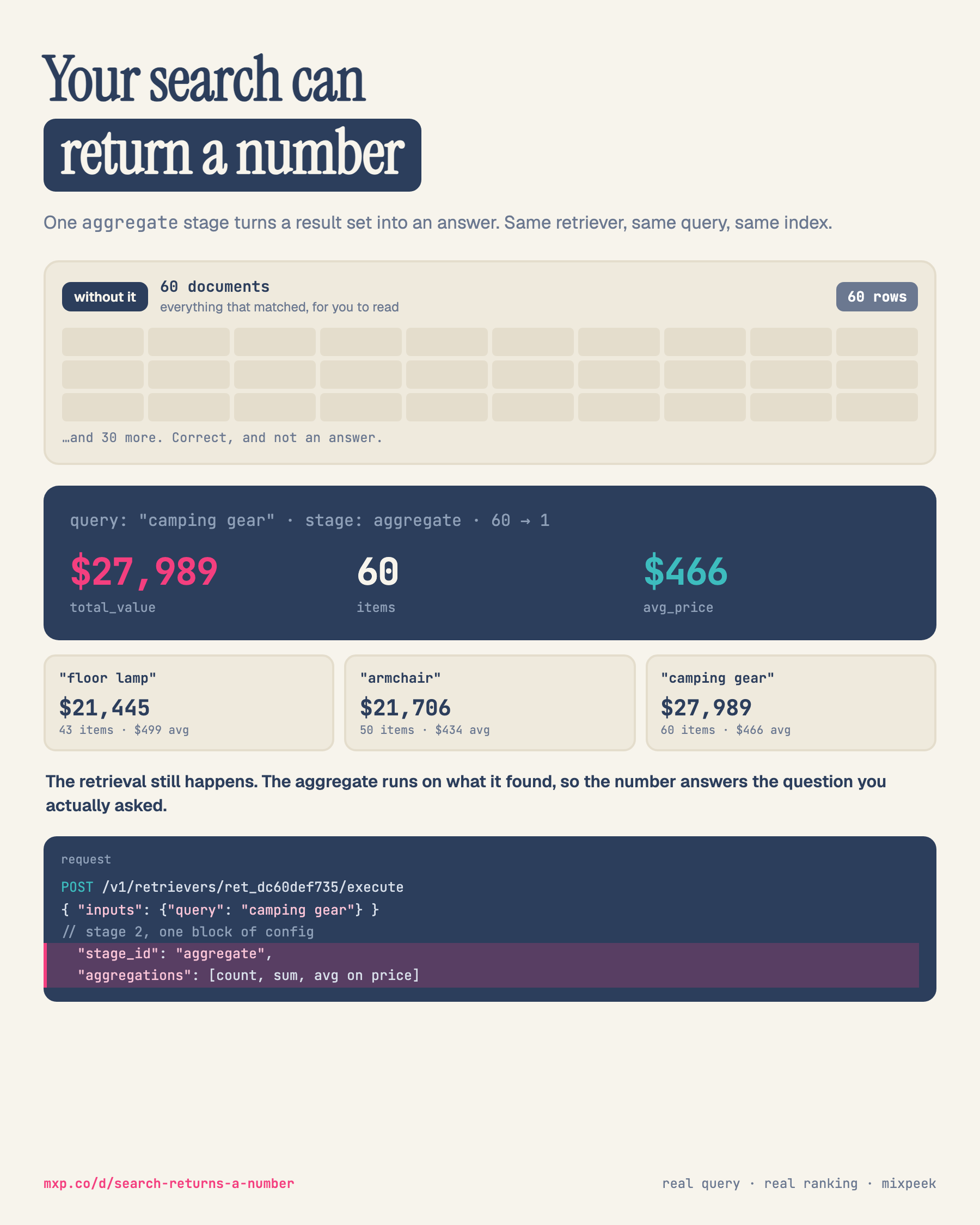
    A portrait diagram. The headline reads Your search can return a number, with the subline: one aggregate stage turns a result set into an answer, same retriever, same query, same index. A rail badged without it shows 60 documents, everything that matched for you to read, drawn as three rows of blank result tiles with the note and 30 more, correct, and not an answer; the chip reads 60 rows. A dark band reads query camping gear, stage aggregate, 60 to 1, with three large figures: 27,989 dollars total_value, 60 items, 466 dollars avg_price. Three smaller cards give the same pipeline on other queries: floor lamp 21,445 dollars across 43 items at 499 average, armchair 21,706 dollars across 50 items at 434 average, camping gear 27,989 dollars across 60 items at 466 average. A bold line states that the retrieval still happens and the aggregate runs on what it found, so the number answers the question you actually asked. A code window shows the execute request with query camping gear and a highlighted second stage, stage_id aggregate with aggregations count, sum and avg on price. The footer prints mxp.co/d/search-returns-a-number.
    Retrieval Mechanics

    Your Search Can Return a Number

    "camping gear" against a 118 image index returns 60 documents. Add one aggregate stage and the same query returns $27,989 across 60 items at $466 average. The retrieval still runs; the aggregate computes over exactly what it found.
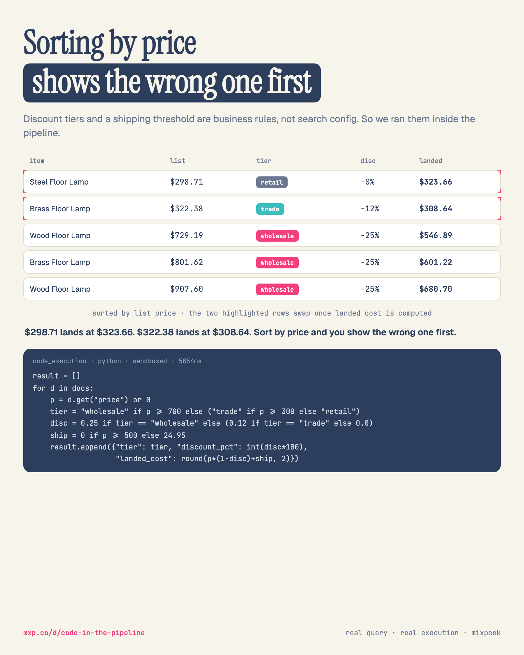
    A portrait diagram. The headline reads Sorting by price, shows the wrong one first, with the subline: discount tiers and a shipping threshold are business rules, not search config, so we ran them inside the pipeline. A five-row table has columns item, list, tier, disc and landed. Steel Floor Lamp, 298.71 dollars, retail, 0 percent, landed 323.66; Brass Floor Lamp, 322.38 dollars, trade, 12 percent, landed 308.64; Wood Floor Lamp, 729.19 dollars, wholesale, 25 percent, landed 546.89; Brass Floor Lamp, 801.62 dollars, wholesale, 25 percent, landed 601.22; Wood Floor Lamp, 907.60 dollars, wholesale, 25 percent, landed 680.70. The first two rows are outlined in rose, with the caption sorted by list price, the two highlighted rows swap once landed cost is computed. A bold line reads 298.71 dollars lands at 323.66, 322.38 dollars lands at 308.64, sort by price and you show the wrong one first. A dark code window labelled code_execution, python, sandboxed, 5854 ms shows the Python that assigns a tier by price, a discount of 25, 12 or 0 percent, free shipping at or above 500 dollars and 24.95 below, and appends tier, discount_pct and landed_cost per document. The footer prints mxp.co/d/code-in-the-pipeline and real query, real execution, mixpeek.
    Retrieval Mechanics

    Sorting by Price Shows the Wrong One First: Landed Cost Computed Inside the Pipeline

    A real "floor lamp" query, then a sandboxed Python stage applies discount tiers and a shipping threshold to each result. $298.71 lands at $323.66 and $322.38 lands at $308.64, so the two cheapest rows swap. Sort by list price and the wrong lamp is first.

    A portrait diagram. The headline reads One photo in, twenty listings out, with the subline explaining that Google Lens reverse image search runs as a stage inside the retriever and returns where a visual match of an asset is listed across the open web. The top band shows the catalog row for a fabric armchair, SKU MXP-CHA-1000 at $446.05, category chair, material fabric, photographed by Pușcaș Adryan on Pexels. Below it one stage labelled external_reverse_image with engine google_lens returns 20 numbered rows of retailers, among them Target, Macy's, Bed Bath & Beyond, Lowe's, The Citizenry, Walmart, World Market, Overstock, Wayfair, Key Home Furnishings, The Home Depot and Castlery, marked as 13 domains. A footer shows the four-line stage config and the live-run date 2026-09-06.
    Retrieval Mechanics

    One Photo In, Twenty Listings Out: Reverse Image Search as a Retriever Stage

    One product photo from a 118-image demo catalog, run through the external_reverse_image stage, came back as 20 ranked retail listings across 13 domains in a single call. Google Lens returns visual matches, so every row is a product that looks like this chair.

    A portrait diagram. The headline reads Your nylon audit needs the backpacks too, with the subline that semantic search matches what a thing looks like, three of these five tents are polyester or canvas, and material is a fact the customer owns, so it lives on a typed edge that one hop follows. The query is nylon camping tent. A feature_search band shows the top five results, two of five nylon: two Nylon Camping Tents, two Polyester Camping Tents and one Canvas Camping Tent, each with its SKU. A traverse_edge band follows same_material from each hit and adds seven Nylon Hiking Backpacks with their SKUs, marked plus seven nylon. A footer shows the edge written on the object, with type same_material and attributes material nylon and target_category backpack, and the stage config with edge_type same_material, direction out, include_source true and max_per_source 7.
    Retrieval Mechanics

    Your Nylon Audit Needs the Backpacks Too: One Edge Hop Inside the Retriever

    "nylon camping tent" over 118 product images returns five tents, and three of them are polyester or canvas. One traverse_edge hop along a customer-owned same_material edge adds the seven nylon hiking backpacks that no image embedding would rank near a tent.
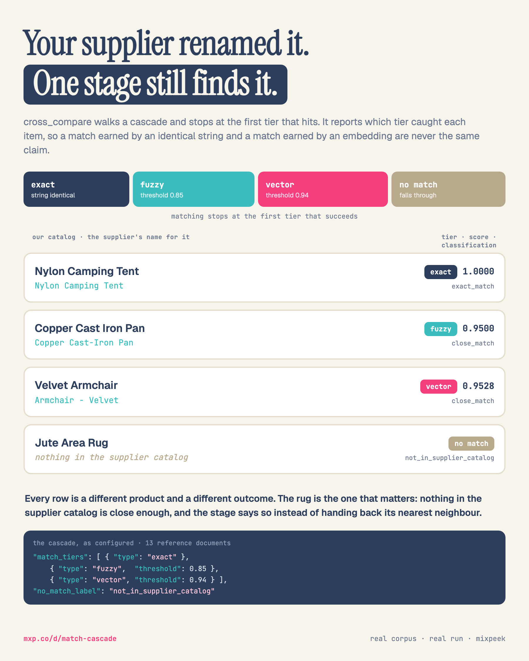
    A portrait diagram. The headline reads Your supplier renamed it, one stage still finds it, with the subline that cross_compare walks a cascade, stops at the first tier that hits and reports which tier caught each item. A band shows the four tiers: exact (string identical), fuzzy (threshold 0.85), vector (threshold 0.94) and no match (falls through). A table pairs four catalog items with the supplier's name for them: Nylon Camping Tent matched exactly at 1.0000 as exact_match; Copper Cast Iron Pan matched Copper Cast-Iron Pan at the fuzzy tier, 0.9500, close_match; Velvet Armchair matched Armchair - Velvet at the vector tier, 0.9528, close_match; Jute Area Rug matched nothing and is labelled not_in_supplier_catalog. A footer shows the configured match_tiers and no_match_label over 13 reference documents.
    Retrieval Mechanics

    Your Supplier Renamed It, One Stage Still Finds It: A Matching Cascade That Reports Its Tier

    Four catalog items reconciled against a 13-item supplier list. An identical string matches at the exact tier, one hyphen falls through to fuzzy at 0.95, a reordered name falls through to vector at 0.9528, and a jute rug that has no counterpart is reported as not_in_supplier_catalog instead of being paired with the nearest wool rug.